Tensorflow内存分配与Keras模型参数

2019独角兽企业重金招聘Python工程师标准>>>

最经典的LeNet模型

MNIST手写体识别的LeNet模型几乎已经成为深度学习玩家耳熟能详，妇孺皆知的模型。所以我们在这里简单的回顾一下，整个模型层次结构如下：

• input输入层
• 卷积核为5x5的conv2d卷积层
• 2x2的Maxpooling池化层
• 卷积核为5x5的conv2d卷积层
• 2x2的Maxpooling池化层
• 1024的full-connect全连接层
• output输出层

MNIST数据集特征张量通常都是（X，28，28，1），那么由上述结构我们可以写出对应的Keras代码，如下代码所示：

from keras.models import Sequential
from keras.layers import Dense, Dropout, Flatten
from keras.layers import Conv2D, MaxPooling2D

model = Sequential()

model.add(Conv2D(32, (5,5), activation='relu', padding='same', input_shape=(28,28,1)))
model.add(MaxPooling2D((2,2)))

model.add(Conv2D(64, (5,5), activation='relu', padding='same'))
model.add(MaxPooling2D((2,2)))

model.add(Flatten())
model.add(Dense(1024, activation='relu'))
model.add(Dropout(0.5))
model.add(Dense(11, activation='softmax'))

Keras框架是一个封装好的深度学习框架，但是Tensorflow框架相对于Keras框架更为底层一些，所以搭建过程相对复杂一些，笔者就直接用Tensorflow官方为我们提供的较为具有公信力的代码mnist_with_summaries.py

将权重设置，偏移值设置，卷积操作，池化操作，参数变化记录，添加层的操作都封装成函数，代码如下：

import tensorflow as tf
import numpy as np

def weight_variable(shape):
    initial = tf.truncated_normal(shape, stddev = 0.1)
    return tf.Variable(initial)

def bias_variable(shape):
    initial = tf.constant(0.1, shape = shape)
    return tf.Variable(initial)

def conv2d(x, W):
    return tf.nn.conv2d(x, W, strides=[1, 1, 1, 1], padding='SAME')

def max_pool_2x2(x):
    return tf.nn.max_pool(x, ksize=[1, 2, 2, 1], strides=[1, 2, 2, 1], padding='SAME')

def variable_summaries(var):
    """Attach a lot of summaries to a Tensor (for TensorBoard visualization)."""
    with tf.name_scope('summaries'):
        mean = tf.reduce_mean(var)
        tf.summary.scalar('mean', mean)
        with tf.name_scope('stddev'):
            stddev = tf.sqrt(tf.reduce_mean(tf.square(var - mean)))
        tf.summary.scalar('stddev', stddev)
        tf.summary.scalar('max', tf.reduce_max(var))
        tf.summary.scalar('min', tf.reduce_min(var))
        tf.summary.histogram('histogram', var)

def add_layer(input_tensor, weights_shape, biases_shape, layer_name, act = tf.nn.relu, flag = 1):
    """Reusable code for making a simple neural net layer.

    It does a matrix multiply, bias add, and then uses relu to nonlinearize.
    It also sets up name scoping so that the resultant graph is easy to read,
    and adds a number of summary ops.
    """
    with tf.name_scope(layer_name):
        with tf.name_scope('weights'):
            weights = weight_variable(weights_shape)
            variable_summaries(weights)
        with tf.name_scope('biases'):
            biases = bias_variable(biases_shape)
            variable_summaries(biases)
        with tf.name_scope('Wx_plus_b'):
            if flag == 1:
                preactivate = tf.add(conv2d(input_tensor, weights), biases)
            else:
                preactivate = tf.add(tf.matmul(input_tensor, weights), biases)
            tf.summary.histogram('pre_activations', preactivate)
        if act == None:
            outputs = preactivate
        else:
            outputs = act(preactivate, name = 'activation')
            tf.summary.histogram('activation', outputs)
        return outputs

with tf.name_scope('Input'):
    x = tf.placeholder(tf.float32, [None, 28*28], name = 'input_x')
    y_ = tf.placeholder(tf.float32, [None, 10], name = 'target_y')

# First Convolutional Layer
x_image = tf.reshape(x, [-1, 28, 28 ,1])
conv_1 = add_layer(x_image, [5, 5, 1, 32], [32], 'First_Convolutional_Layer', flag = 1)

# First Pooling Layer
pool_1 = max_pool_2x2(conv_1)

# Second Convolutional Layer 
conv_2 = add_layer(pool_1, [5, 5, 32, 64], [64], 'Second_Convolutional_Layer', flag = 1)

# Second Pooling Layer 
pool_2 = max_pool_2x2(conv_2)

# Densely Connected Layer
pool_2_flat = tf.reshape(pool_2, [-1, 7*7*64])
dc_1 = add_layer(pool_2_flat, [7*7*64, 1024], [1024], 'Densely_Connected_Layer', flag = 0) 

# Dropout
keep_prob = tf.placeholder(tf.float32)
dc_1_drop = tf.nn.dropout(dc_1, keep_prob)

# Readout Layer
y = add_layer(dc_1_drop, [1024, 10], [10], 'Readout_Layer', flag = 0)

本文的重点并不是如何搭建MNIST深度学习模型，所以，对于损失函数和优化器的选择本文并未详细列出，这个问题笔者有研究过，详见之前篇博客深度学习的核心——分类器的选择，这篇博客中针对深度学习中激活函数的使用和优化器选择有详细解释。

Keras模型参数

很多用过Keras平台的深度学习玩家在搭建深度学习模型后会习惯性的使用一条语句model.summary()，这条语句的作用是将我们之前用代码搭建的模型用表格的形式展现出来。这个表格包括如下内容：模型层结构的名称、这层对应输出的张量Tensor以及这层运算产生的参数。下图所对应是上面Keras搭建MNIST模型后，调用model.summary()这条语句所打印的模型信息。很多玩家会用这条语句测试模型是否出现问题，笔者百度之后没有发现这个参数Param这些数字理论依据，所以，笔者在这里说明这些参数的由来。

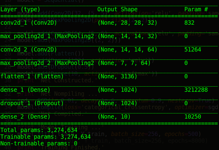
我们不妨首先看全连接层的参数由来：

10250 = 1024×10+1×10

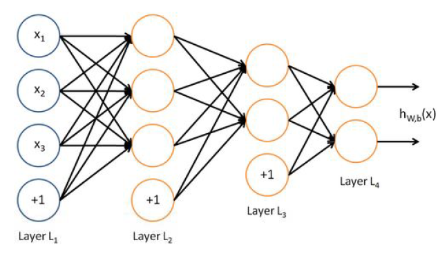
这个式子并不是在凑数，其本质的原因是，我们在最后一个全连接层，也就是我们的输出层的前一层设置10个神经元，上层设置的神经元1024个神经元要与本层的10个神经元全部连接，此时产生1024×10个参数。我们都知道，机器学习或深度学习中，一个核心的公式是：Y=WX+b，依据这个道理，我们每层都要有一个偏移值b，所以此时产生了1×10个参数，整个这一层产生的参数是1024×10+1×10=10250个。同理上一个全连接层参数3212288=3136×1024+1×1024 ，下图是笔者在模式识别课中，神经网络中多层感知器的神经元连接图，读者可以根据所学的知识计算一下总共的神经元数量，笔者算得如下结果，这是一个三个隐层的网络，总共有7个神经元。

读者会问，卷积层又是如何计算呢？卷积层存在参数共享的特性，什么是参数共享呢？参数共享（parameter sharing）是指在一个模型的多个函数中使用相同的参数。在传统的神经网络中，当计算一层的输出时，权重矩阵的每一个元素只使用一次，当它乘以输入的一个元素后就再也不会用到了。作为参数共享的同义词，我们可以说一个网络含有绑定的权重（tied weights），因为用于一个输入的权重也会被绑定在其他的权重上。在卷积神经网络中，核的每一个元素都作用在输入的每一位置上（是否考虑边界像素取决于对边界决策的设计）。卷积运算中的参数共享保证了我们只需要学习一个参数集合，而不是对于每一位置都需要学习一个单独的参数集合。根据这个原理我们可以的如下计算方法

832=（5×5×1+1）×32

其中5×5是我们定义的卷积核大小，第一个1是输入的通道数，第二个1是常数，意义为那个偏移值，32是输出通道数的大小。同理对于第二层卷积51264=（5×5×32+1）×64 。当我们们计算完卷积和全连接的所有参数后，将其相加就可以获得总的参数。

Tensorflow内存参数

tf.RunOptions()，tf.RunMetadata()是重要的记录Tensorflow运行计算过程中所用的计算时间和Memeroy，我们用MNIST数据集中一条数据来测试显示出每一层进行运算时所包括的参数信息，这里我们读取已经训练好的Tensorflow pb模型。其中pb模型将整个Tensorflow运算和训练的权值都存入到pb文件中，代码如下：

from tensorflow.python.platform import gfile
from tensorflow.examples.tutorials.mnist import input_data

import numpy as np
import tensorflow as tf
import mnist_inference

mnist_data_path = 'MNIST_data/'
mnist = input_data.read_data_sets(mnist_data_path, one_hot = True)
batch_xs, batch_ys = mnist.test.images[:1], mnist.test.labels[:1]
print batch_ys.shape

with tf.Session() as sess:
    with tf.device('/cpu:0'):

        with gfile.FastGFile('LeNet_mnist.pb','rb') as f:
            graph_def = tf.GraphDef()
            graph_def.ParseFromString(f.read())
        sess.run(tf.global_variables_initializer())
        tf.import_graph_def(graph_def, name='')

        input_tensor = sess.graph.get_tensor_by_name('input:0')
        output = sess.graph.get_tensor_by_name('layer6-fc2/output:0')
        
        y_ = tf.placeholder(tf.float32,[None,10], name = 'target')
        drop_rate = sess.graph.get_tensor_by_name('dropout:0')
        correct_prediction = tf.equal(tf.argmax(output,1),tf.argmax(y_,1))
        accuracy = tf.reduce_mean(tf.cast(correct_prediction,tf.float32))
        tf.summary.scalar('accuracy', accuracy)
        merged = tf.summary.merge_all()
        
        test_writer = tf.summary.FileWriter('pbtest', sess.graph)
        run_options = tf.RunOptions(trace_level=tf.RunOptions.FULL_TRACE)
        run_metadata = tf.RunMetadata()
        _, test_accuracy = sess.run([merged, accuracy], feed_dict={input_tensor: batch_xs, y_: batch_ys, drop_rate:1.0},
                                                     options=run_options,
                                                     run_metadata=run_metadata)
        test_writer.add_run_metadata(run_metadata, "test_process")
        test_writer.close()
        

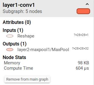
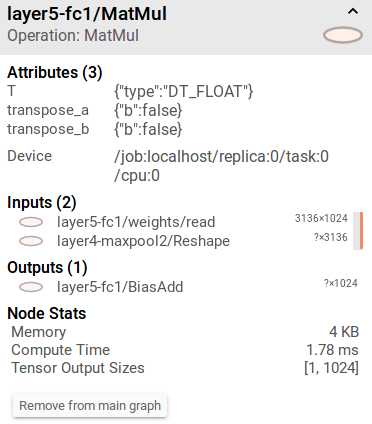
如下图是Tensorboard中Graph对应点击模型每一层展现的对应信息，其中包括Inputs，Outputs，Node Stats（Memory和Compute Time）。内存分配是Tensorflow中一个重要的模块，但在这里的内存分配还是比较容易理解的，Tensorflow在这里的内存分配笔者认为分配给输出的内存，保证进行这一层操作后输出有足够的内存。所以，笔者认为其内存的大小是这样定义的

98KB=98×1024B=28×28×32×4B

如何理解？我们的输出Tensor是28×28×32，由于我们的Tensor定义的是float类型的值，float这种类型的变量分配4个字节的内存空间

同理我们的第二层卷积的内存分配

49KB=49×1024B=14×14×64×4B

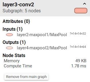
那么我们的全连接层的内存分配：4KB=4×1024B=1024×4B

还想再聊聊

笔者并非刻意研究分享什么内容，而是在实际科研学习实践的过程中，发现一些比较小型，很多人未解决或大牛们懒的解决的点，并将其研究解释清楚。

如果有问题和对这个感兴趣的朋友留言给我，下面是我的邮箱

nextowang@stu.xidian.edu.cn

感谢阅读，期待您的反馈！

 

 

转载于:https://my.oschina.net/nextowang/blog/1031545