


1: Neural Networks And Iris Flowers
Many machine learning prediction problems are rooted in complex data and its non-linear relationships between features. Neural networks are a class of models that can learn these non-linear interactions between variables.
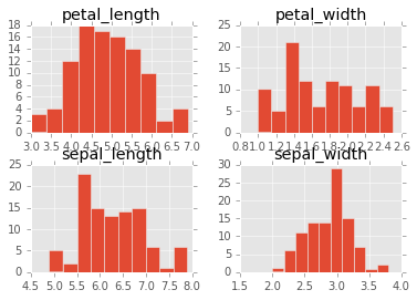
We will introduce neural networks by predicting the species of iris flowers from data with the following features:
sepal_length- Continuous variable measured in centimeters.sepal_width- Continuous variable measured in centimeters.petal_length- Continuous variable measured in centimeters.petal_width- Continuous variable measured in centimeters.species- Categorical. 2 species of iris flowers, Iris-virginica or Iris-versicolor.
The DataFrame class includes a hist() method which creates a histogram for every numeric column in that DataFrame. The histograms are generated using Matplotlib and displayed using plt.show().
Instructions
- Visualize the data using the method
hist()on our DataFrameirisand showing the plots.
import pandas
import matplotlib.pyplot as plt
import numpy as np
# Read in dataset
iris = pandas.read_csv("iris.csv")
# shuffle rows
shuffled_rows = np.random.permutation(iris.index)
iris = iris.loc[shuffled_rows,:]
print(iris.head())
# There are 2 species
print(iris.species.unique())
iris.hist()
plt.show()
2: Neurons
So far we have talked about methods which do not allow for a large amount of non-linearity. For example, in the two dimensional case shown below, we want to find a function that can cleanly seperate the X's from the O's.
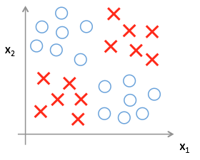
Neither a linear model nor logistic model is capable of building such a function, so we must explore other options like neural networks. Neural networks are very loosely inspired by the structure of neurons in the human brain. These models are built by using a series of activation units, known as neurons, to make predictions of some outcome. Neurons take in some input, apply a transformation function, and return an output. Below we see a representation of a neuron.
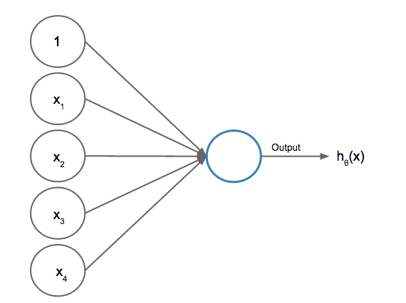
This neuron is taking in 5 units represented as xx, a bias unit, and 4 features. This bias unit (1) is similar in concept to the intercept in linear regression and it will shift the activity of the neuron to one direction or the other. These units are then fed into an activation function hh. We will use the popular sigmoid (logistic) activation function because it returns values between 0 and 1 and can be treated as probabilities.
Sigmoid Function: 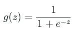
This sigmoid function then leads to the corresponding activation function:
Sigmoid Activation Function: 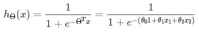
If you look closely, you might notice that the logistic regression function we learned in previous lessons can be represented here as a neuron.
Instructions
- Write a function called
sigmoid_activationwith inputsxa feature vector andthetaa parameter vector of the same length to implement the sigmoid activation function.- Assign the value of
sigmoid_activation(x0, theta_init)toa1.a1should be a vector.
- Assign the value of
z = np.asarray([[9, 5, 4]])
y = np.asarray([[-1, 2, 4]])
# np.dot is used for matrix multiplication
# z is 1x3 and y is 1x3, z * y.T is then 1x1
print(np.dot(z,y.T))
# Variables to test sigmoid_activation
iris["ones"] = np.ones(iris.shape[0])
X = iris[['ones', 'sepal_length', 'sepal_width', 'petal_length', 'petal_width']].values
y = (iris.species == 'Iris-versicolor').values.astype(int)
# The first observation
x0 = X[0]
# Initialize thetas randomly
theta_init = np.random.normal(0,0.01,size=(5,1))
def sigmoid_activation(x, theta):
x = np.asarray(x)
theta = np.asarray(theta)
return 1 / (1 + np.exp(-np.dot(theta.T, x)))
a1 = sigmoid_activation(x0, theta_init)
3: Cost Function
We can train a single neuron as a two layer network using gradient descent. As we learned in the previous mission, we need to minimize a cost function which measures the error in our model. The cost function measures the difference between the desired output and actual output, defined as:
J(Θ)=−1m∑mi=1(yi∗log(hΘ(xi))+(1−yi)log(1−hΘ(xi)))J(Θ)=−1m∑i=1m(yi∗log(hΘ(xi))+(1−yi)log(1−hΘ(xi)))
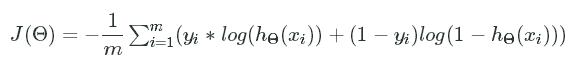
Since our targets, yiyi , are binary, either yiyi or (1−yi)(1−yi)
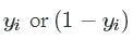 will equal zero. One of the terms in the summation will disappear because of this result and. the activation function is then used to compute the error. For example, if we observe a true target, yi=1yi=1
 , then we want hΘ(xi)hΘ(xi)
 to also be close to 1. So as hΘ(xi)hΘ(xi)
  approaches 1, the log(hΘ(xi))log(hΘ(xi))
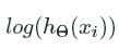 becomes very close to 0. Since the log of a value between 0 and 1 is negative, we must take the negative of the entire summation to compute the cost. The parameters are randomly initialized using a normal random variable with a small variance, less than 0.1.
Instructions
- Write a function,
singlecost(), that can compute the cost from just a single observation.- This function should use input features
X, targetsy, and parametersthetato compute the cost function. - Assign the cost of variables
x0,y0, andtheta_initto variablefirst_cost.
- This function should use input features
# First observation's features and target
x0 = X[0]
y0 = y[0]
# Initialize parameters, we have 5 units and just 1 layer
theta_init = np.random.normal(0,0.01,size=(5,1))
def singlecost(X, y, theta):
# Compute activation
h = sigmoid_activation(X.T, theta)
# Take the negative average of target*log(activation) + (1-target) * log(1-activation)
cost = -np.mean(y * np.log(h) + (1-y) * np.log(1-h))
return cost
first_cost = singlecost(x0, y0, theta_init)
4: Compute The Gradients
In the previous mission we learned that we need to compute the partial deriviatives of the cost function to get the gradients. Calculating derivatives are more complicated in neural networks than in linear regression. Here we must compute the overall error and then distribute that error to each parameter. Compute the derivative using the chain rule.
∂J∂θj=∂J∂h(Θ)∂h(Θ)∂θj∂J∂θj=∂J∂h(Θ)∂h(Θ)∂θj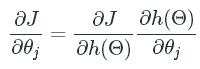
This rule may look complicated, but we can break it down. The first part is computing the error between the target variable and prediction. The second part then computes the sensitivity relative to each parameter. In the end, the gradients are computed as: δ=(yi−hΘ(xi))∗hΘ(xi)∗(1−hΘ(xi))∗xiδ=(yi−hΘ(xi))∗hΘ(xi)∗(1−hΘ(xi))∗xi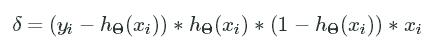 .
.
Now we will step through the math. (yi−hΘ(xi))(yi−hΘ(xi))![]() is a scalar and the error between our target and prediction. hΘ(xi)∗(1−hΘ(xi))hΘ(xi)∗(1−hΘ(xi))
is a scalar and the error between our target and prediction. hΘ(xi)∗(1−hΘ(xi))hΘ(xi)∗(1−hΘ(xi))![]() is also a scalar and the sensitivity of the activation function. xixi is the features for our observation i. δδ is then a vector of length 5, 4 features plus a bias unit, corresponding to the gradients.
is also a scalar and the sensitivity of the activation function. xixi is the features for our observation i. δδ is then a vector of length 5, 4 features plus a bias unit, corresponding to the gradients.
To implement this, we compute δδ![]() for each observation, then average to get the average gradient. The average gradient is then used to update the corresponding parameters.
for each observation, then average to get the average gradient. The average gradient is then used to update the corresponding parameters.
Instructions
- Compute the average gradients over each observation in
Xand corresponding targetywith the initialized parameterstheta_init.- Assign the average gradients to variable
grads.
- Assign the average gradients to variable
# Initialize parameters
theta_init = np.random.normal(0,0.01,size=(5,1))
# Store the updates into this array
grads = np.zeros(theta_init.shape)
# Number of observations
n = X.shape[0]
for j, obs in enumerate(X):
# Compute activation
h = sigmoid_activation(obs, theta_init)
# Get delta
delta = (y[j]-h) * h * (1-h) * obs
# accumulate
grads += delta[:,np.newaxis]/X.shape[0]
5: Two Layer Network
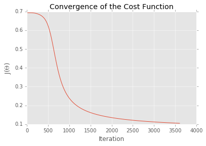
Now that you can compute the gradients, use gradient descent to learn the parameters and predict the species of iris flower given the 4 features. Gradient descent minimizes the cost function by adjusting the parameters accordingly. Adjust the parameters by substracting the product of the gradients and the learning rate from the previous parameters. Repeat until the cost function coverges or a maximum number of iterations is reached.
The high level algorithm is,
while (number_of_iterations < max_iterations and (prev_cost - cost) > convergence_thres ) {
update paramaters
get new cost
repeat
}
We have implemented all these pieces in a single function learn() that can learn this two layer network. After setting a few initial variables, we begin to iterate until convergence. During each iteration we compute our gradients, update accordingly, and compute the new cost.
Instructions
This step is a demo. Play around with code or advance to the next step.
theta_init = np.random.normal(0,0.01,size=(5,1))
# set a learning rate
learning_rate = 0.1
# maximum number of iterations for gradient descent
maxepochs = 10000
# costs convergence threshold, ie. (prevcost - cost) > convergence_thres
convergence_thres = 0.0001
def learn(X, y, theta, learning_rate, maxepochs, convergence_thres):
costs = []
cost = singlecost(X, y, theta) # compute initial cost
costprev = cost + convergence_thres + 0.01 # set an inital costprev to past while loop
counter = 0 # add a counter
# Loop through until convergence
for counter in range(maxepochs):
grads = np.zeros(theta.shape)
for j, obs in enumerate(X):
h = sigmoid_activation(obs, theta) # Compute activation
delta = (y[j]-h) * h * (1-h) * obs # Get delta
grads += delta[:,np.newaxis]/X.shape[0] # accumulate
# update parameters
theta += grads * learning_rate
counter += 1 # count
costprev = cost # store prev cost
cost = singlecost(X, y, theta) # compute new cost
costs.append(cost)
if np.abs(costprev-cost) < convergence_thres:
break
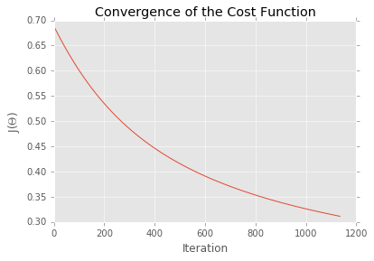
plt.plot(costs)
plt.title("Convergence of the Cost Function")
plt.ylabel("J($\Theta$)")
plt.xlabel("Iteration")
plt.show()
return theta
theta = learn(X, y, theta_init, learning_rate, maxepochs, convergence_thres)
6: Neural Network
Neural networks are usually built using mulitple layers of neurons. Adding more layers into the network allows you to learn more complex functions. Here's a picture representing a 3 layer neural network.
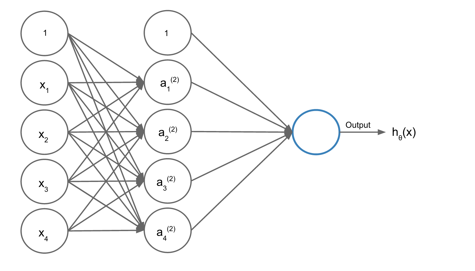
We have a 3 layer neural network with four input variables ![]() , and
, and ![]() and a bias unit. Each variable and bias unit is then sent to four hidden units,
and a bias unit. Each variable and bias unit is then sent to four hidden units, ![]() . The hidden units have different sets of parameters
. The hidden units have different sets of parameters ![]() .
.
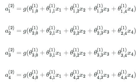
![]() represents the parameter of input unit kk which transform the units in layer jj to activation unit
represents the parameter of input unit kk which transform the units in layer jj to activation unit  .
.
This layer is known as a hidden layer because the user does not directly interact with it by passing or retrieving data. The third and final layer is the output, or prediction, of our model. Similar to how each variable was sent to each neuron in the hidden layer, the activation units in each neuron are then sent to each neuron on the next layer. Since there is only a single layer, we can write it as:
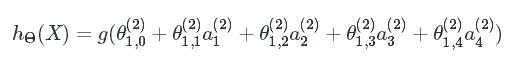
While the mathematical notation may seem confusing at first, at a high level, we are organizing multiple logistic regression models to create a more complex function.
Instructions
- Write a function
feedforward()that will take in an inputXand two sets of parameterstheta0andtheta1to compute the output
- Assign the output to variable
husing featuresXand parameterstheta0_initandtheta1_init.
- Assign the output to variable
theta0_init = np.random.normal(0,0.01,size=(5,4))
theta1_init = np.random.normal(0,0.01,size=(5,1))
def feedforward(X, theta0, theta1):
# feedforward to the first layer
a1 = sigmoid_activation(X.T, theta0).T
# add a column of ones for bias term
a1 = np.column_stack([np.ones(a1.shape[0]), a1])
# activation units are then inputted to the output layer
out = sigmoid_activation(a1.T, theta1)
return out
h = feedforward(X, theta0_init, theta1_init)
7: Multiple Neural Network Cost Function
The cost function to multiple layer neural networks is identical to the cost function we used in the last screen, but hΘ(xi)hΘ(xi)![]() is more complicated.
is more complicated.
J(Θ)=−1m∑mi=1(yi∗log(hΘ(xi))+(1−yi)log(1−hΘ(xi))J(Θ)=−1m∑i=1m(yi∗log(hΘ(xi))+(1−yi)log(1−hΘ(xi))![]()
Instructions
- Write a function
multiplecost()which estimates the cost function.- Use the observations in
X, targetsyand inital parameterstheta0_initandtheta1_init. - Assign the cost to variable
c.
- Use the observations in
theta0_init = np.random.normal(0,0.01,size=(5,4))
theta1_init = np.random.normal(0,0.01,size=(5,1))
# X and y are in memory and should be used as inputs to multiplecost()
def multiplecost(X, y, theta0, theta1):
# feed through network
h = feedforward(X, theta0, theta1)
# compute error
inner = y * np.log(h) + (1-y) * np.log(1-h)
# negative of average error
return -np.mean(inner)
c = multiplecost(X, y, theta0_init, theta1_init)
8: Backpropagation
Now that we have mulitple layers of parameters to learn, we must implement a method called backpropagation. We've already implemented forward propagation by feeding the data through each layer and returning an output. Backpropagation focuses on updating parameters starting at the last layer and circling back through each layer, updating accordingly. As there are multiple layers we are forced to compute ∂∂Θ(l)i,jJ(Θ)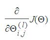 where l is the layer. For a three layer network, use the following approach,
δlj![]() is the 'error' for unit j in layer l
is the 'error' for unit j in layer l
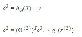
There is no δ1 since the first layer are the features and have no error.
We have written code that trains a three layer neural network in the code cell. You will notice that there are many parameters and moving parts to this algorithm. To make the code more modular, we have refactored our previous code as a class, allowing us to organize related attributes and methods.
We have reused feedforward() and multiplecost() but in more condensed forms. During initialization, we set attributes like the learning rate, maximum number of iterations to convergence, and number of units in the hidden layer. In learn() you'll find the backpropagation algorithm, which computes the gradients and updates the parameters. We then test the class by using the features and thespecies of the flower.
Instructions
This step is a demo. Play around with code or advance to the next step.
# Use a class for this model, it's good practice and condenses the code
class NNet3:
def __init__(self, learning_rate=0.5, maxepochs=1e4, convergence_thres=1e-5, hidden_layer=4):
self.learning_rate = learning_rate
self.maxepochs = int(maxepochs)
self.convergence_thres = 1e-5
self.hidden_layer = int(hidden_layer)
def _multiplecost(self, X, y):
# feed through network
l1, l2 = self._feedforward(X)
# compute error
inner = y * np.log(l2) + (1-y) * np.log(1-l2)
# negative of average error
return -np.mean(inner)
def _feedforward(self, X):
# feedforward to the first layer
l1 = sigmoid_activation(X.T, self.theta0).T
# add a column of ones for bias term
l1 = np.column_stack([np.ones(l1.shape[0]), l1])
# activation units are then inputted to the output layer
l2 = sigmoid_activation(l1.T, self.theta1)
return l1, l2
def predict(self, X):
_, y = self._feedforward(X)
return y
def learn(self, X, y):
nobs, ncols = X.shape
self.theta0 = np.random.normal(0,0.01,size=(ncols,self.hidden_layer))
self.theta1 = np.random.normal(0,0.01,size=(self.hidden_layer+1,1))
self.costs = []
cost = self._multiplecost(X, y)
self.costs.append(cost)
costprev = cost + self.convergence_thres+1 # set an inital costprev to past while loop
counter = 0 # intialize a counter
# Loop through until convergence
for counter in range(self.maxepochs):
# feedforward through network
l1, l2 = self._feedforward(X)
# Start Backpropagation
# Compute gradients
l2_delta = (y-l2) * l2 * (1-l2)
l1_delta = l2_delta.T.dot(self.theta1.T) * l1 * (1-l1)
# Update parameters by averaging gradients and multiplying by the learning rate
self.theta1 += l1.T.dot(l2_delta.T) / nobs * self.learning_rate
self.theta0 += X.T.dot(l1_delta)[:,1:] / nobs * self.learning_rate
# Store costs and check for convergence
counter += 1 # Count
costprev = cost # Store prev cost
cost = self._multiplecost(X, y) # get next cost
self.costs.append(cost)
if np.abs(costprev-cost) < self.convergence_thres and counter > 500:
break
# Set a learning rate
learning_rate = 0.5
# Maximum number of iterations for gradient descent
maxepochs = 10000
# Costs convergence threshold, ie. (prevcost - cost) > convergence_thres
convergence_thres = 0.00001
# Number of hidden units
hidden_units = 4
# Initialize model
model = NNet3(learning_rate=learning_rate, maxepochs=maxepochs,
convergence_thres=convergence_thres, hidden_layer=hidden_units)
# Train model
model.learn(X, y)
# Plot costs
plt.plot(model.costs)
plt.title("Convergence of the Cost Function")
plt.ylabel("J($\Theta$)")
plt.xlabel("Iteration")
plt.show()
9: Splitting Data
Now that we have learned about neural networks, learned about backpropagation, and have code which will train a 3-layer neural network, we will split the data into training and test datasets and run the model.
Instructions
- Choose the first 70 rows in both
Xandyand assign them respectively toX_trainandy_train.
# First 70 rows to X_train and y_train
# Last 30 rows to X_train and y_train
X_train = X[:70]
y_train = y[:70]
X_test = X[-30:]
y_test = y[-30:]
10: Predicting Iris Flowers
To benchmark how well a three layer neural network performs when predicting the species of iris flowers, you will have to compute the AUC, area under the curve, score of the receiver operating characteristic. The function NNet3 not only trains the model but also returns the predictions. The method predict() will return a 2D matrix of probabilities. Since there is only one target variable in this neural network, select the first row of this matrix, which corresponds to the type of flower.
Instructions
- Train the neural network using
X_testandy_testandmodel, which has been initialized with a set of parameters. - Once training is complete, use the
predict()function to return the probabilities of the flower matching thespeciesIris-versicolor. - Compute the AUC score, using
roc_auc_score()and assign it toauc.
from sklearn.metrics import roc_auc_score
# Set a learning rate
learning_rate = 0.5
# Maximum number of iterations for gradient descent
maxepochs = 10000
# Costs convergence threshold, ie. (prevcost - cost) > convergence_thres
convergence_thres = 0.00001
# Number of hidden units
hidden_units = 4
# Initialize model
model = NNet3(learning_rate=learning_rate, maxepochs=maxepochs,
convergence_thres=convergence_thres, hidden_layer=hidden_units)
model.learn(X_train, y_train)
yhat = model.predict(X_test)[0]
auc = roc_auc_score(y_test, yhat)


 1739
1739

 被折叠的 条评论
为什么被折叠?
被折叠的 条评论
为什么被折叠?
 到【灌水乐园】发言


