Kaggle比赛系列: (4) House Prices: Advanced Regression Techniques

声明: 从kaggle入门比赛的第4篇开始,将不会再详细的贴出数据处理\特征工程\建模流程,针对每一片文章的特点,突出leaf在大神notebook中的主要收获,但是完整代码我依然会打包整理上传.

1. drop(inplace)剔除某一列

train.drop("Id", axis = 1, inplace = True)
test.drop("Id", axis = 1, inplace = True)

使用DataFrame.drop()函数时,对于 inplace 参数, 默认情况下取值为False ,作用为:不在原数据中更改.这时的结果依然是DataFrame数据类型,所以可以写成例如 train = train.drop(“Id”, axis = 1, [inplace = False]) 的形式.但是当inplace参数为True时,返回的值类型为Nonetype,不能再赋值给train,所以只能写成train.drop(“Id”, axis = 1, inplace = True) 的形式.

2. train.drop(train[select case].index)剔除某一行

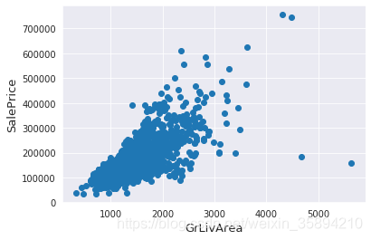
#Deleting outliers
train = train.drop(train[(train['GrLivArea']>4000) & (train['SalePrice']<300000)].index)

注意这里的作用是:将训练集中 GrLivArea>4000和SalePrice<300000 的数据清除记录(行),容易错误的写成
train = train.drop(((train[‘GrLivArea’]>4000) & (train[‘SalePrice’]<300000)).index) 即在对DataFrame进行某一属性的筛选时,应该将筛选条件放在**[ ]**中.
在剔除异常数据记录时应注意: There are probably others outliers in the training data. However, removing all them may affect badly our models if ever there were also outliers in the test data. That’s why , instead of removing them all, we will just manage to make some of our models robust on them. You can refer to the modelling part of this notebook for that.
剔除一小部分严重异常的数据,对剩下的依然存在异常数据的数据集进行建模,能够增强模型的鲁帮性.

3.分布直方图绘制(拟合曲线,正态分布曲线)

sns.distplot(train['SalePrice'] , fit=norm);#绘制拟合曲线和正态分布曲线

# Get the fitted parameters used by the function
(mu, sigma) = norm.fit(train['SalePrice'])#获得正态分布的平均值和方差
print( '\n mu = {:.2f} and sigma = {:.2f}\n'.format(mu, sigma))

#Now plot the distribution
plt.legend(['Normal dist. ($\mu=$ {:.2f} and $\sigma=$ {:.2f} )'.format(mu, sigma)],
            loc='best')#$\mu=$是一个转意方法, loc= 'best'是常用的标签排版的方法
plt.ylabel('Frequency')
plt.title('SalePrice distribution')

#Get also the QQ-plot
fig = plt.figure()
res = stats.probplot(train['SalePrice'], plot=plt)
plt.show()

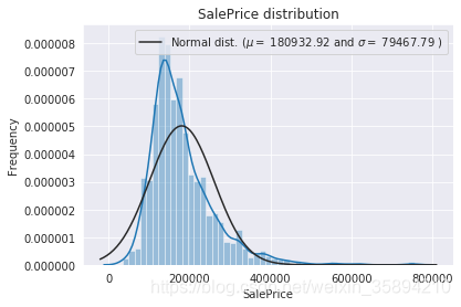
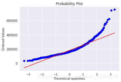
由图可见,售价的分布是偏峰(左)的,(skew值较大),需要变化成为更加正态化的分布.

#We use the numpy fuction log1p which  applies log(1+x) to all elements of the column
train["SalePrice"] = np.log1p(train["SalePrice"])#将偏峰转化为正态分布

4. 数据集合并(pd.concat)

all_data = pd.concat((train, test)).reset_index(drop=True)#数据集合并
all_data.drop(['SalePrice'], axis=1, inplace=True)#删除某一列

数据集合并方法pd.concat((train, test).reset_index(drop=True))

5. 查看缺失数据集的比例

all_data_na = (all_data.isnull().sum() / len(all_data)) * 100
all_data_na = all_data_na.drop(all_data_na[all_data_na == 0].index).sort_values(ascending=False)[:30]
missing_data = pd.DataFrame({'Missing Ratio' :all_data_na})
missing_data.head(20)

(1) all_data.isnull().sum() 会对DataFrame中的每一列进行统计;
(2) pd.DataFrame({‘Missing Ratio’: all_data_na}) 为DataFrame中的某一列设置字段名,注意是以字典的形式.

6.缺失值填充

(1)

all_data['PoolQC'] = all_data['PoolQC'].fillna("None")#None填充

(2)

all_data['LotFrontage'] = all_data.groupby("Neiborhood")["LotFrontage"].transform(lambda x: x.fillna(x.median()))#分组transform(lambda)取中值

(3)

for col in ('GarageType', 'GarageFinish', 'GarageQual', 'GarageCond'):
    all_data[col] = all_data[col].fillna('None')

(4)

all_data['MSZoning'] = all_data['MSZoning'].fillna(all_data['MSZoning'].mode()[0])#使用众数填充缺失值

7. 标签编码

什么是独热编码和标签编码

from sklearn.preprocessing import LabelEncoder
cols = ('FireplaceQu', 'BsmtQual', 'BsmtCond', 'GarageQual', 'GarageCond', 
        'ExterQual', 'ExterCond','HeatingQC', 'PoolQC', 'KitchenQual', 'BsmtFinType1', 
        'BsmtFinType2', 'Functional', 'Fence', 'BsmtExposure', 'GarageFinish', 'LandSlope',
        'LotShape', 'PavedDrive', 'Street', 'Alley', 'CentralAir', 'MSSubClass', 'OverallCond',
        'YrSold', 'MoSold')
# process columns, apply LabelEncoder to categorical features
for c in cols:
    lbl = LabelEncoder() 
    lbl.fit(list(all_data[c].values)) 
    all_data[c] = lbl.transform(list(all_data[c].values))

fit()学习编码 + transform()进行编码

8.求数值型属性的偏度

numeric_feats = all_data.dtypes[all_data.dtypes != "object"].index

# Check the skew of all numerical features
skewed_feats = all_data[numeric_feats].apply(lambda x: skew(x.dropna())).sort_values(ascending=False)#需要首先x.dropna()
print("\nSkew in numerical features: \n")
skewness = pd.DataFrame({'Skew' :skewed_feats})
skewness.head(10)

对偏度进行矫正:
(Note that setting λ=0 is equivalent to log1p used above for the target variable.)

skewness = skewness[abs(skewness) > 0.75]
print("There are {} skewed numerical features to Box Cox transform".format(skewness.shape[0]))

from scipy.special import boxcox1p
skewed_features = skewness.index
lam = 0.15
for feat in skewed_features:
    #all_data[feat] += 1
    all_data[feat] = boxcox1p(all_data[feat], lam)
    
#all_data[skewed_features] = np.log1p(all_data[skewed_features])

9. 将类别属性拆开分别作为一个属性

all_data = pd.get_dummies(all_data)

10.设计交叉验证方法

n_folds = 5

def rmsle_cv(model):
	kf = KFold(n_folds, shuffle=True, random_state = 42).get_n_splits(train.values)
	rmse = np.sqrt(-cross_val_score(model, train.values, y_train,scoreing="neg_mean_squared_error", cv = kf))
	return(rmse)

cross_val_score()是一种模型训练方法, 传入参数为:机器学习模型\训练数据集\标签\损失函数
最后的 cv = kf是要求采用n折交叉验证的方法作为最终的结果

11.模型设计与测试

例: LASSO Regression
模型特点:对异常值敏感,可采用sklearn中的Robustscaler()方法应用于LASSO的pipeline上,使其更具鲁棒性.

lasso = make_pipeline(RobustScaler(), Lasso(alpha = 0.0005, random_state = 1))

测试: score = rmsle_cv(lasso)
结果: Lasso score: 0.1115 (0.0074)

12. 模型集成

(1) 简单的集成方法: 对基础模型取平均值

class AveragingModels(BaseEstimator, RegressorMixin, TransformerMixin):
    def __init__(self, models):
        self.models = models
        
    # we define clones of the original models to fit the data in
    def fit(self, X, y):
        self.models_ = [clone(x) for x in self.models]
        
        # Train cloned base models
        for model in self.models_:
            model.fit(X, y)

        return self
    
    #Now we do the predictions for cloned models and average them
    def predict(self, X):
        predictions = np.column_stack([
            model.predict(X) for model in self.models_
        ])
        return np.mean(predictions, axis=1)   

测试:

averaged_models = AveragingModels(models = (ENet, GBoost, KRR, lasso))
score = rmsle_cv(averaged_models)

(2) 采用元模型的模型集成方法

训练过程如下:
a. 将训练集拆分成没有交叉的两部分(train和holdout部分);
b. 在train数据集上训练基础模型
c. 在holdout数据集上测试基础模型
d. 将步骤©中的每个模型的测试结果作为输入,以target variable作为输出训练更高层的"元模型"
对stacking的解释可以参考:添加链接描述

class StackingAveragedModels(BaseEstimator, RegressorMixin, TransformerMixin):
    def __init__(self, base_models, meta_model, n_folds=5):
        self.base_models = base_models
        self.meta_model = meta_model
        self.n_folds = n_folds
   
    # We again fit the data on clones of the original models
    def fit(self, X, y):
        self.base_models_ = [list() for x in self.base_models]
        self.meta_model_ = clone(self.meta_model)
        kfold = KFold(n_splits=self.n_folds, shuffle=True, random_state=156)
        
        # Train cloned base models then create out-of-fold predictions
        # that are needed to train the cloned meta-model
        out_of_fold_predictions = np.zeros((X.shape[0], len(self.base_models)))
        for i, model in enumerate(self.base_models):
            for train_index, holdout_index in kfold.split(X, y):
                instance = clone(model)
                self.base_models_[i].append(instance)
                instance.fit(X[train_index], y[train_index])
                y_pred = instance.predict(X[holdout_index])
                out_of_fold_predictions[holdout_index, i] = y_pred
                
        # Now train the cloned  meta-model using the out-of-fold predictions as new feature
        self.meta_model_.fit(out_of_fold_predictions, y)
        return self
   
    #Do the predictions of all base models on the test data and use the averaged predictions as 
    #meta-features for the final prediction which is done by the meta-model
    def predict(self, X):
        meta_features = np.column_stack([
            np.column_stack([model.predict(X) for model in base_models]).mean(axis=1)
            for base_models in self.base_models_ ])
        return self.meta_model_.predict(meta_features)

测试:

stacked_averaged_models = StackingAveragedModels(base_models = (ENet, GBoost, KRR),meta_model = lasso)
score = rmsle_cv(stacked_averaged_models)

(3) Ensembling 融合模型 + XGBoost + LightGBM

(1) 定义评价指标

def rmsle(y, y_pred):
    return np.sqrt(mean_squared_error(y, y_pred))

(2) Ensembling模型分别预测

model_lgb.fit(train, y_train)
lgb_train_pred = model_lgb.predict(train)
lgb_pred = np.expm1(model_lgb.predict(test.values))
print(rmsle(y_train, lgb_train_pred))

(3) Ensembling在训练集上预测

rmsle(y_train,stacked_train_pred*0.70 + xgb_train_pred*0.15 + lgb_train_pred*0.15 )

(4) Ensemble prediction

ensemble = stacked_pred*0.70 + xgb_pred*0.15 + lgb_pred*0.15

数据集下载: https://pan.baidu.com/s/1dGDNVIx1RiSyHVWfNayrMg 提取码: axx6
源码:https://pan.baidu.com/s/1l_acggNRYSFxAZrqnqoBdQ 提取码: nsm4