吴恩达机器学习课程第七周笔记

最新推荐文章于 2022-10-08 12:01:30 发布

DreamHigh_GRT

最新推荐文章于 2022-10-08 12:01:30 发布

阅读量556

点赞数

分类专栏：机器学习文章标签：吴恩达机器学习课程笔记

本文链接：https://blog.csdn.net/weixin_37501173/article/details/95035705

版权

机器学习专栏收录该内容

1 篇文章 0 订阅

订阅专栏

吴恩达机器学习课程第七周笔记

超参数调试、Batch正则化和程序框架（Hyperparameter tuning）
Programming assignment

超参数调试、Batch正则化和程序框架（Hyperparameter tuning）

自己学习时记下的一些笔记， ^ _ ^!!

2019.7.8
独立实现一个自己想要的功能的网络

调试处理（Tuning process）

在这里插入图片描述
众多的超参数调整时有不同的优先级，上图中按照红色、橙色、紫色的顺序调整。不同的算法又有不同的参数，有些参数使用的数值很少需要作出调整。例如Momentum参数 $\beta$ ，0.9就是个很好的默认值。调试mini-batch的大小，可以使最优算法运行有效。还会经常调试隐藏单元，用橙色圈住的这些，这三个是其次比较重要的，相对于而言。重要性排第三位的是其他因素，层数有时会产生很大的影响，学习率衰减也是如此。当应用Adam算法时, $\beta1$ , $\beta2$ 和 $\varepsilon$ ，总是选定其分别为0.9，0.999和10^-8。
在这里插入图片描述
在深度学习领域，通常采用随机选择点的方法，因为对于特定的问题而言，很难提前知道哪个超参数最重要，如果采用网格的选点方式，可能会有很多点浪费掉。

当在局部某些点处取得较好结果后，在其周边范围进行精细调整。

为超参数选择合适的范围（Using an appropriate scale to pick hyperparameters）

在这里插入图片描述
有时用对数标尺搜索超参数的方式会更合理，如果你在10^a和10^b之间取值，在此例中，a即-4，b即0。你要做的就是在[a,b]区间随机均匀地给r取值，这个例子中r\in[-4,0]，然后你可以设置a的值，然后设置a的值，基于随机取样的超参数a=10^r。有时也为 $\beta$ =1-10^r。
因为当 $\beta$ 接近1时，所得结果的灵敏度会变化，即使有微小的变化。所以 $\beta$ 在0.9到0.9005之间取值，无关紧要，你的结果几乎不会变化。
在这里插入图片描述

超参数调试实践：Pandas VS Caviar（Hyperparameters tuning in practice: Pandas vs. Caviar）

在这里插入图片描述
如今的深度学习已经应用到许多不同的领域，某个应用领域的超参数设定，有可能通用于另一领域，不同的应用领域出现相互交融。比如，我曾经看到过计算机视觉领域中涌现的巧妙方法，比如说Confonets或ResNets，这我们会在后续课程中讲到。它还成功应用于语音识别，我还看到过最初起源于语音识别的想法成功应用于NLP等等。
就超参数的设定而言，我见到过有些直觉想法变得很缺乏新意，所以，即使你只研究一个问题，比如说逻辑学，你也许已经找到一组很好的参数设置，并继续发展算法，或许在几个月的过程中，观察到你的数据会逐渐改变，或也许只是在你的数据中心更新了服务器，正因为有了这些变化，你原来的超参数的设定不再好用，所以我建议，重新测试或评估你的超参数，至少每隔几个月一次，以确保你对数值依然很满意。
在这里插入图片描述
一种是一次照看一个模型，另一种方法则是同时试验多种模型。像熊猫照看孩子，或是鱼子酱的方式。

归一化网络的激活函数（Normalizing activations in a network）

在这里插入图片描述
常做的是归一化z而不是a。Batch归一化的作用是它适用的归一化过程，不只是输入层，甚至同样适用于神经网络中的深度隐藏层。你应用Batch归一化了一些隐藏单元值中的平均值和方差，不过训练输入和这些隐藏单元值的一个区别是，你也许不想隐藏单元值必须是平均值0和方差1。
如果你有sigmoid激活函数，你不想让你的值总是全部集中在这里，你想使它们有更大的方差，或不是0的平均值，以便更好的利用非线性的sigmoid函数，而不是使所有的值都集中于这个线性版本中，这就是为什么有了和两个参数后，你可以确保所有的值可以是你想赋予的任意值，或者它的作用是保证隐藏的单元已使均值和方差标准化。那里，均值和方差由两参数控制，即 $\gamma$ 和 $\beta$ ，学习算法可以设置为任何值，所以它真正的作用是，使隐藏单元值的均值和方差标准化，即有固定的均值和方差，均值和方差可以是0和1，也可以是其它值，它是由 $\gamma$ 和 $\beta$ 两参数控制的。

将 Batch Norm 拟合进神经网络（Fitting Batch Norm into a neural network）

深度网络训练中的Batch Norm
在这里插入图片描述
Batch归一化学习参数 $\beta1$ ， $\beta2$ 等等和用于Momentum、Adam、RMSprop算法中的 $\beta$ 不同。
例如，对于给定层，会计算d $\beta$ ^[l]，接着更新参数 $\beta$ 为 $\beta$ ^[l]- $\alpha$ d $\beta$ ^[l]。你也可以使用Adam或RMSprop或Momentum，以更新参数和，并不是只应用梯度下降法。
先将z^[l]归一化，结果为均值0和标准方差，再由 $\beta$ 和 $\gamma$ 重缩放，但这意味着，无论b^[l]的值是多少，都是要被减去的。b^[l]这个参数没有意义，所以可以去掉。
在这里插入图片描述

Batch Norm 为什么奏效？（Why does Batch Norm work?）

在这里插入图片描述

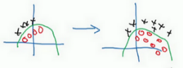
“Covariate shift”，想法是这样的，如果你已经学习了x到y的映射，如果x的分布改变了，那么你可能需要重新训练你的学习算法。
在这里插入图片描述
输入数据均值和方差变化巨大，会对训练权重产生难度。
原因一：Batch 归一化减少了输入值改变的问题，使参数更稳定
原因二：Batch 归一化有轻微的正则化效果，因为标准差的缩放和减去均值带来额外噪声，而Mini-batch使标准差与均匀值同样有误差，因此具有轻微正则化作用。
Batch归一化一次只能处理一个Mini-batch数据，它在mini-batch上计算均值和方差。所以测试时最好使用训练时没有使用过的样本，以确保预测有意义。

测试时的 Batch Norm（Batch Norm at test time）

在整个训练集上可以用指数加权平均等方法为 $\mu$ 和 $\sigma$ ²

Softmax 回归（Softmax regression）

在这里插入图片描述

训练一个 Softmax 分类器（Training a Softmax classifier）

那么反向传播步骤或者梯度下降法又如何呢？其实初始化反向传播所需要的关键步骤或者说关键方程是这个表达式dz^[l]=y_hat-y。
在这里插入图片描述
有了这个，你就可以计算，然后开始反向传播的过程，计算整个神经网络中所需要的所有导数。

深度学习框架（Deep Learning frameworks）

在这里插入图片描述
选择框架的标准。
一个重要的标准就是便于编程，这既包括神经网络的开发和迭代，还包括为产品进行配置，为了成千上百万，甚至上亿用户的实际使用，取决于你想要做什么。
第二个重要的标准是运行速度，特别是训练大数据集时，一些框架能让你更高效地运行和训练神经网络。
还有一个标准人们不常提到，也很重要，那就是这个框架是否真的开放，要是一个框架真的开放，它不仅需要开源，而且需要良好的管理。不幸的是，在软件行业中，一些公司有开源软件的历史，但是公司保持着对软件的全权控制，当几年时间过去，人们开始使用他们的软件时，一些公司开始逐渐关闭曾经开放的资源，或将功能转移到他们专营的云服务中。因此值得注意的一件事就是你能否相信这个框架能长时间保持开源，而不是在一家公司的控制之下，它未来有可能出于某种原因选择停止开源，即便现在这个软件是以开源的形式发布的。但至少在短期内，取决于你对语言的偏好，看你更喜欢Python，Java还是C++或者其它什么，也取决于你在开发的应用，是计算机视觉，还是自然语言处理或者线上广告，等等。

TensorFlow

Programming assignment

1. Exploring the Tensorflow Library

import math
import numpy as np
import h5py
import matplotlib.pyplot as plt
import tensorflow as tf
from tensorflow.python.framework import ops
from tf_utils import load_dataset, random_mini_batches, convert_to_one_hot, predict

%matplotlib inline
np.random.seed(1)

Writing and running programs in TensorFlow has the following steps:

1.Create Tensors (variables) that are not yet executed/evaluated.

y_hat = tf.constant(36, name='y_hat')            # Define y_hat constant. Set to 36.
y = tf.constant(39, name='y')                    # Define y. Set to 39

2.Write operations between those Tensors.

loss = tf.Variable((y - y_hat)**2, name='loss')  # Create a variable for the loss

3.Initialize your Tensors.

init = tf.global_variables_initializer()         # When init is run later (session.run(init)),
                                                 # the loss variable will be initialized and ready to be computed

4.Create a Session.
5.Run the Session. This will run the operations you’d written above.

with tf.Session() as session:                    # Create a session and print the output
    session.run(init)                            # Initializes the variables
    print(session.run(loss))                     # Prints the loss

例一：

a = tf.constant(2)
b = tf.constant(10)
c = tf.multiply(a,b)
sess = tf.Session()
print(sess.run(c))

例二：

x = tf.placeholder(tf.int64, name = 'x')
sess = tf.Session()
print(sess.run(2 * x, feed_dict = {x: 3}))
sess.close()

1.1 - Linear function

TensorFlow实现一个Y=WX+b的线性方程的计算，向量内部数字为随机数。

def linear_function():
    """
    Implements a linear function: 
            Initializes W to be a random tensor of shape (4,3)
            Initializes X to be a random tensor of shape (3,1)
            Initializes b to be a random tensor of shape (4,1)
    Returns: 
    result -- runs the session for Y = WX + b 
    """
    
    np.random.seed(1)
    
    ### START CODE HERE ### (4 lines of code)
    X = tf.constant(np.random.randn(3,1), name = "X")
    W = tf.constant(np.random.randn(4,3), name = "W")
    b = tf.constant(np.random.randn(4,1), name = "b")
    Y = tf.constant(np.random.randn(4,1), name = "Y")
    ### END CODE HERE ### 
    
    # Create the session using tf.Session() and run it with sess.run(...) on the variable you want to calculate
    
    ### START CODE HERE ###
    sess = tf.Session()
    result = sess.run(tf.matmul(W,X)+b)
    ### END CODE HERE ### 
    
    # close the session 
    sess.close()

    return result

1.2 - Computing the sigmoid

激活函数sigmoid的实现方法：函数内部声明一个占位符x，声明一个运算sigmoid作为运算符，将传入参数，通过feed_dict在函数内部运行session对其进行计算。

def sigmoid(z):
    """
    Computes the sigmoid of z
    
    Arguments:
    z -- input value, scalar or vector
    
    Returns: 
    results -- the sigmoid of z
    """
    
    ### START CODE HERE ### ( approx. 4 lines of code)
    # Create a placeholder for x. Name it 'x'.
    x = tf.placeholder(tf.float32, name = "x")

    # compute sigmoid(x)
    sigmoid = tf.sigmoid(x)

    # Create a session, and run it. Please use the method 2 explained above. 
    # You should use a feed_dict to pass z's value to x. 
    with tf.Session() as sess: 
        # Run session and call the output "result"
        result = sess.run(sigmoid, feed_dict = {x: z})
    
    ### END CODE HERE ###
    
    return result

1.3 - Computing the Cost

Implement the cross entropy loss. The function you will use is:

tf.nn.sigmoid_cross_entropy_with_logits(logits = …, labels = …)

def cost(logits, labels):
    """
    Computes the cost using the sigmoid cross entropy
    
    Arguments:
    logits -- vector containing z, output of the last linear unit (before the final sigmoid activation)
    labels -- vector of labels y (1 or 0) 
    
    Note: What we've been calling "z" and "y" in this class are respectively called "logits" and "labels" 
    in the TensorFlow documentation. So logits will feed into z, and labels into y. 
    
    Returns:
    cost -- runs the session of the cost (formula (2))
    """
    
    ### START CODE HERE ### 
    
    # Create the placeholders for "logits" (z) and "labels" (y) (approx. 2 lines)
    z = tf.placeholder(tf.float32, name = "z")
    y = tf.placeholder(tf.float32, name = "y")
    
    # Use the loss function (approx. 1 line)
    cost = tf.nn.sigmoid_cross_entropy_with_logits(logits =z,  labels = y)
    
    # Create a session (approx. 1 line). See method 1 above.
    sess = tf.Session()
    
    # Run the session (approx. 1 line).
    cost = sess.run(cost,feed_dict = {z:logits,y:labels})
    
    # Close the session (approx. 1 line). See method 1 above.
    sess.close()
    
    ### END CODE HERE ###
    
    return cost

1.4 - Using One Hot encodings

在这里插入图片描述
将标签数字改为One Hot编码，所用tensorflow函数为：

tf.one_hot(labels, depth, axis)

def one_hot_matrix(labels, C):
    """
    Creates a matrix where the i-th row corresponds to the ith class number and the jth column
                     corresponds to the jth training example. So if example j had a label i. Then entry (i,j) 
                     will be 1. 
                     
    Arguments:
    labels -- vector containing the labels 
    C -- number of classes, the depth of the one hot dimension
    
    Returns: 
    one_hot -- one hot matrix
    """
    
    ### START CODE HERE ###
    
    # Create a tf.constant equal to C (depth), name it 'C'. (approx. 1 line)
    C = tf.constant(C, name = "C")
    
    # Use tf.one_hot, be careful with the axis (approx. 1 line)
    one_hot_matrix = tf.one_hot(labels, C,axis=0)
    
    # Create the session (approx. 1 line)
    sess = tf.Session()
    
    # Run the session (approx. 1 line)
    one_hot = sess.run(one_hot_matrix)
    
    # Close the session (approx. 1 line). See method 1 above.
    sess.close()
    
    ### END CODE HERE ###
    
    return one_hot

1.5 - Initialize with zeros and ones

how to initialize a vector of zeros and ones.

tf.ones(shape)
tf.zeros(shape)

def ones(shape):
    """
    Creates an array of ones of dimension shape
    
    Arguments:
    shape -- shape of the array you want to create
        
    Returns: 
    ones -- array containing only ones
    """
    
    ### START CODE HERE ###
    
    # Create "ones" tensor using tf.ones(...). (approx. 1 line)
    ones = tf.ones(shape)
    
    # Create the session (approx. 1 line)
    sess = tf.Session()
    
    # Run the session to compute 'ones' (approx. 1 line)
    ones = sess.run(ones)
    
    # Close the session (approx. 1 line). See method 1 above.
    sess.close()
    
    ### END CODE HERE ###
    return ones

2 . Building your first neural network in tensorflow

2.0 - Problem statement: SIGNS Dataset

Training set: 1080 pictures (64 by 64 pixels) of signs representing numbers from 0 to 5 (180 pictures per number).
Test set: 120 pictures (64 by 64 pixels) of signs representing numbers from 0 to 5 (20 pictures per number).

数据集使用流程

# 加载数据集Loading the dataset
X_train_orig, Y_train_orig, X_test_orig, Y_test_orig, classes = load_dataset()
# 将图片数据向量化Flatten the training and test images 
X_train_flatten = X_train_orig.reshape(X_train_orig.shape[0], -1).T
X_test_flatten = X_test_orig.reshape(X_test_orig.shape[0], -1).T
# Normalize image vectors
X_train = X_train_flatten/255.
X_test = X_test_flatten/255.
# 将图片标签进行one hot 处理Convert training and test labels to one hot matrices
Y_train = convert_to_one_hot(Y_train_orig, 6)
Y_test = convert_to_one_hot(Y_test_orig, 6)

2.1 - Create placeholders
为神经网络的输入X，输出Y创建占位符。由于输入层神经元个数和标签种类是确定的，而每个batch输入样本的数量是不确定的，由此可以分别将X、Y的shape设置为(n_x,None)、(n_y,None)。

def create_placeholders(n_x, n_y):
    """
    Creates the placeholders for the tensorflow session.
    
    Arguments:
    n_x -- scalar, size of an image vector (num_px * num_px = 64 * 64 * 3 = 12288)
    n_y -- scalar, number of classes (from 0 to 5, so -> 6)
    
    Returns:
    X -- placeholder for the data input, of shape [n_x, None] and dtype "float"
    Y -- placeholder for the input labels, of shape [n_y, None] and dtype "float"
    
    Tips:
    - You will use None because it let's us be flexible on the number of examples you will for the placeholders.
      In fact, the number of examples during test/train is different.
    """

    ### START CODE HERE ### (approx. 2 lines)
    X = tf.placeholder(tf.float32,(n_x,None) ,name = "Placeholder_1")
    Y = tf.placeholder(tf.float32,(n_y,None), name = "Placeholder_2")
    ### END CODE HERE ###
    
    return X, Y

2.2 - Initializing the parameters

初始化权重：

W1 = tf.get_variable(“W1”, [25,12288], initializer = tf.contrib.layers.xavier_initializer(seed = 1))
b1 = tf.get_variable(“b1”, [25,1], initializer = tf.zeros_initializer())
不太清楚tf.contrib.layers.xavier_initializer（）函数初始化的具体细节，据说Xavier是用于初始化权重，并使每一层的梯度大小相似。

def initialize_parameters():
    """
    Initializes parameters to build a neural network with tensorflow. The shapes are:
                        W1 : [25, 12288]
                        b1 : [25, 1]
                        W2 : [12, 25]
                        b2 : [12, 1]
                        W3 : [6, 12]
                        b3 : [6, 1]
    
    Returns:
    parameters -- a dictionary of tensors containing W1, b1, W2, b2, W3, b3
    """
    
    tf.set_random_seed(1)                   # so that your "random" numbers match ours
        
    ### START CODE HERE ### (approx. 6 lines of code)
    W1 = tf.get_variable("W1", [25,12288], initializer = tf.contrib.layers.xavier_initializer(seed = 1))
    b1 = tf.get_variable("b1", [25,1], initializer = tf.zeros_initializer())
    W2 = tf.get_variable("W2", [12, 25], initializer = tf.contrib.layers.xavier_initializer(seed = 1))
    b2 = tf.get_variable("b2", [12, 1], initializer = tf.zeros_initializer())
    W3 = tf.get_variable("W3", [6, 12], initializer = tf.contrib.layers.xavier_initializer(seed = 1))
    b3 = tf.get_variable("b3", [6, 1], initializer = tf.zeros_initializer())
    ### END CODE HERE ###

    parameters = {"W1": W1,
                  "b1": b1,
                  "W2": W2,
                  "b2": b2,
                  "W3": W3,
                  "b3": b3}
    
    return parameters

2.3 - Forward propagation in tensorflow

前向传递，计算A[i]与Z[i]至Z3，等待Z3用于softmax。

def forward_propagation(X, parameters):
    """
    Implements the forward propagation for the model: LINEAR -> RELU -> LINEAR -> RELU -> LINEAR -> SOFTMAX
    
    Arguments:
    X -- input dataset placeholder, of shape (input size, number of examples)
    parameters -- python dictionary containing your parameters "W1", "b1", "W2", "b2", "W3", "b3"
                  the shapes are given in initialize_parameters

    Returns:
    Z3 -- the output of the last LINEAR unit
    """
    
    # Retrieve the parameters from the dictionary "parameters" 
    W1 = parameters['W1']
    b1 = parameters['b1']
    W2 = parameters['W2']
    b2 = parameters['b2']
    W3 = parameters['W3']
    b3 = parameters['b3']
    
    ### START CODE HERE ### (approx. 5 lines)              # Numpy Equivalents:
    Z1 = tf.add(tf.matmul(W1,X),b1)                                            # Z1 = np.dot(W1, X) + b1
    A1 = tf.nn.relu(Z1)                                              # A1 = relu(Z1)
    Z2 = tf.add(tf.matmul(W2,A1),b2)                                              # Z2 = np.dot(W2, a1) + b2
    A2 = tf.nn.relu(Z2)                                            # A2 = relu(Z2)
    Z3 = tf.add(tf.matmul(W3,A2),b3)                                                 # Z3 = np.dot(W3,Z2) + b3
    ### END CODE HERE ###
    
    return Z3

2.4 Compute cost

计算损失函数的方法，其中先用Z3计算softmax,再计算交叉熵，tf.reduce_mean()对整个交叉熵的返回向量取了平均值得到cost。

tf.reduce_mean(tf.nn.softmax_cross_entropy_with_logits(logits = …, labels = …))
tf.reduce_mean()
tf.reduce_mean()用于计算张量tensor沿着指定的数轴（tensor的某一维度）上的的平均值，主要用作降维或者计算tensor（图像）的平均值，默认对所有的元素求平均。

# GRADED FUNCTION: compute_cost 

def compute_cost(Z3, Y):
    """
    Computes the cost
    
    Arguments:
    Z3 -- output of forward propagation (output of the last LINEAR unit), of shape (6, number of examples)
    Y -- "true" labels vector placeholder, same shape as Z3
    
    Returns:
    cost - Tensor of the cost function
    """
    
    # to fit the tensorflow requirement for tf.nn.softmax_cross_entropy_with_logits(...,...)
    logits = tf.transpose(Z3)
    labels = tf.transpose(Y)
    
    ### START CODE HERE ### (1 line of code)
    cost = tf.reduce_mean(tf.nn.softmax_cross_entropy_with_logits(logits=logits,labels = labels))
    ### END CODE HERE ###
    
    return cost

tf.reduce_mean()的详细解释：

该部分引至CSDN 作者：拼命先生A
原文：https://blog.csdn.net/kevindree/article/details/87028948

reduce_mean(input_tensor,
                axis=None,
                keepdims=False,
                name=None,
                reduction_indices=None)
 
#第一个参数 input_tensor： 输入待降维的tensor;
#第二个参数 axis： 指定的维，如果不指定，则计算所有元素的均值;
#第三个参数 keepdims：是否保持原有张量的维度，设置为True，输出的结果保持输入tensor的形状，设置为False，输出结果会降低维度;
#第四个参数 name： 操作的名称，在graph中可使用;

import tensorflow as tf

x = [[1,2,3],
    [1,2,3]]

xx = tf.cast(x,tf.float32)

mean_all = tf.reduce_mean(xx, keepdims=False)
mean_0 = tf.reduce_mean(xx, axis=0, keepdims=False)
mean_1 = tf.reduce_mean(xx, axis=1, keepdims=False)


with tf.Session() as sess:
   m_a,m_0,m_1 = sess.run([mean_all, mean_0, mean_1])

print(m_a)
print(m_0)
print(m_1)


###  输出结果为 ###
# 2.0
# [ 1.  2.  3.]
# [ 2.  2.]

如果设置保持原来张量的维度，keepdims=True ，结果：

### 保持原有张量的维度，设置keepdims=True，输出结果为 ###
# [[2.]]
# [[1. 2. 3.]]
# [[2.] [2.]]

2.5 - Backward propagation & parameter updates

optimizer = tf.train.GradientDescentOptimizer(learning_rate = learning_rate).minimize(cost)
#该运算调用时，必须和cost一起调用，只一行代码，所有反向传递和参数更新都被tensorflow集成进这一函数
_ , c = sess.run([optimizer, cost], feed_dict={X: minibatch_X, Y: minibatch_Y})

2.6 - Building the model
model函数生成训练完毕的深度神经网络的流程：
清除每次运行前default graph 中的节点，并将整张图重置。
set_random_seed()
创建张量和运算：
        获取数据集的数据维度n_x和n_y
        建立cost动态数组，用于存储每训练5步的epoch_cost数据，便于观察损失函数变化。
        创建占位符X和Y
        初始化权重及偏置，这一步相当于明确了网络的层数和每一层的神经元
        创建前向传递的运算
        创建了损失函数的计算
        创建了优化器，需传入学习率参数
        创建了init运算，将通过tf.global_variables_initializer()函数，将所有变量的赋值过程全部run一遍，否则部分张量会出现未被赋值的情况。
创建一个会话，用来进行图计算
        运行init运算
        建立for循环，按照epochs规定的次数进行迭代
                计算mini_batches的个数，划分mini_batch,初始化epoch_cost=0,在每一个epoch中，对mini_batches逐一进行运算,将所有mini_batch的误差求平均得epoch_cos
                        由mini_batch获得minibatch_X和minibatch_Y，会话中运行sess.run([optimizer, cost], feed_dict={X: minibatch_X, Y: minibatch_Y})，在每一个mini_batch计算中更新epoch_cost。
                计算mini_batches的个数，划分mini_batch,初始化epoch_cost=0,在每一个epoch中，对mini_batches逐一进行运算,将所有mini_batch的误差求平均得epoch_cos
                如果epoch次数为整百，打印epoch_cost观察损失函数变化，epoch_cost每训练5个epoch,就向cost数组中增添新的epoch_cost记录
        绘制cost损失函数变化图像。（其中用到了np.squeeze（）函数，用于数组的形状中删除单维度条目，即把shape中为1的维度去掉）
        通过sess.run(parameters)函数，将parameters输出，保存下来，parameters所含内容为整个网络的权重和偏置，同样包含整个神经网络层和每层的神经元的数量信息，parameters即为训练好的神经网络的参数信息。与前向传递的激活函数、Batch_Norm、正则化、输出层激活函数如softmax、损失函数、反向传递的梯度下降法、Momentum、RMSprop、Adam、learning rate decay等其中算法结合，即为整个神经网络的架构。
        通过tf.equal(tf.argmax(Z3), tf.argmax(Y))，tf.reduce_mean(tf.cast(correct_prediction, “float”))两个函数计算模型在测试集上的准确率
        返回模型的parameters

def model(X_train, Y_train, X_test, Y_test, learning_rate = 0.0001,
          num_epochs = 1500, minibatch_size = 32, print_cost = True):
    """
    Implements a three-layer tensorflow neural network: LINEAR->RELU->LINEAR->RELU->LINEAR->SOFTMAX.
    
    Arguments:
    X_train -- training set, of shape (input size = 12288, number of training examples = 1080)
    Y_train -- test set, of shape (output size = 6, number of training examples = 1080)
    X_test -- training set, of shape (input size = 12288, number of training examples = 120)
    Y_test -- test set, of shape (output size = 6, number of test examples = 120)
    learning_rate -- learning rate of the optimization
    num_epochs -- number of epochs of the optimization loop
    minibatch_size -- size of a minibatch
    print_cost -- True to print the cost every 100 epochs
    
    Returns:
    parameters -- parameters learnt by the model. They can then be used to predict.
    """
    
    ops.reset_default_graph()                         # to be able to rerun the model without overwriting tf variables
    tf.set_random_seed(1)                             # to keep consistent results
    seed = 3                                          # to keep consistent results
    (n_x, m) = X_train.shape                          # (n_x: input size, m : number of examples in the train set)
    n_y = Y_train.shape[0]                            # n_y : output size
    costs = []                                        # To keep track of the cost
    
    # Create Placeholders of shape (n_x, n_y)
    ### START CODE HERE ### (1 line)
    X= tf.placeholder(tf.float32,shape=(n_x,None),name="X")
    Y= tf.placeholder(tf.float32,shape=(n_y,None),name="Y")
    ### END CODE HERE ###

    # Initialize parameters
    ### START CODE HERE ### (1 line)
    parameters = initialize_parameters()
    ### END CODE HERE ###
    
    # Forward propagation: Build the forward propagation in the tensorflow graph
    ### START CODE HERE ### (1 line)
    Z3 = forward_propagation(X, parameters)
    ### END CODE HERE ###
    
    # Cost function: Add cost function to tensorflow graph
    ### START CODE HERE ### (1 line)
    cost = compute_cost(Z3, Y)
    ### END CODE HERE ###
    
    # Backpropagation: Define the tensorflow optimizer. Use an AdamOptimizer.
    ### START CODE HERE ### (1 line)
    optimizer = tf.train.GradientDescentOptimizer(learning_rate = learning_rate).minimize(cost)
    ### END CODE HERE ###
    
    # Initialize all the variables
    init = tf.global_variables_initializer()

    # Start the session to compute the tensorflow graph
    with tf.Session() as sess:
        
        # Run the initialization
        sess.run(init)
        
        # Do the training loop
        for epoch in range(num_epochs):

            epoch_cost = 0.                       # Defines a cost related to an epoch
            num_minibatches = int(m / minibatch_size) # number of minibatches of size minibatch_size in the train set
            seed = seed + 1
            minibatches = random_mini_batches(X_train, Y_train, minibatch_size, seed)

            for minibatch in minibatches:

                # Select a minibatch
                (minibatch_X, minibatch_Y) = minibatch
                
                # IMPORTANT: The line that runs the graph on a minibatch.
                # Run the session to execute the "optimizer" and the "cost", the feedict should contain a minibatch for (X,Y).
                ### START CODE HERE ### (1 line)
                _ , minibatch_cost = sess.run([optimizer, cost], feed_dict={X: minibatch_X, Y: minibatch_Y})
                ### END CODE HERE ###
                
                epoch_cost += minibatch_cost / num_minibatches

            # Print the cost every epoch
            if print_cost == True and epoch % 100 == 0:
                print ("Cost after epoch %i: %f" % (epoch, epoch_cost))
            if print_cost == True and epoch % 5 == 0:
                costs.append(epoch_cost)
                
        # plot the cost
        plt.plot(np.squeeze(costs))
        plt.ylabel('cost')
        plt.xlabel('iterations (per tens)')
        plt.title("Learning rate =" + str(learning_rate))
        plt.show()

        # lets save the parameters in a variable
        parameters = sess.run(parameters)
        print ("Parameters have been trained!")

        # Calculate the correct predictions
        correct_prediction = tf.equal(tf.argmax(Z3), tf.argmax(Y))

        # Calculate accuracy on the test set
        accuracy = tf.reduce_mean(tf.cast(correct_prediction, "float"))

        print ("Train Accuracy:", accuracy.eval({X: X_train, Y: Y_train}))
        print ("Test Accuracy:", accuracy.eval({X: X_test, Y: Y_test}))
        
        return parameters

TensorFlow 总结

What you should remember:

Tensorflow is a programming framework used in deep learning
The two main object classes in tensorflow are Tensors and Operators.
When you code in tensorflow you have to take the following steps:
- Create a graph containing Tensors (Variables, Placeholders …) and Operations (tf.matmul, tf.add, …)
- Create a session
- Initialize the session
- Run the session to execute the graph
You can execute the graph multiple times as you’ve seen in model()
The backpropagation and optimization is automatically done when running the session on the “optimizer” object.

DreamHigh_GRT

关注

0
点赞
踩
0

收藏

觉得还不错? 一键收藏
0
评论
吴恩达机器学习课程第七周笔记

吴恩达机器学习课程第七周笔记Hyperparameter tuning,Batch Normalization and Programming FrameworksHyperparameter tuningTuning processUsing an appropriate scale to pick hyperparametersHyperparameters tuning in practic...
复制链接

扫一扫