Python搭建神经网络

   

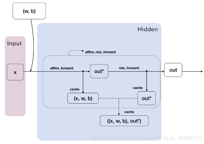
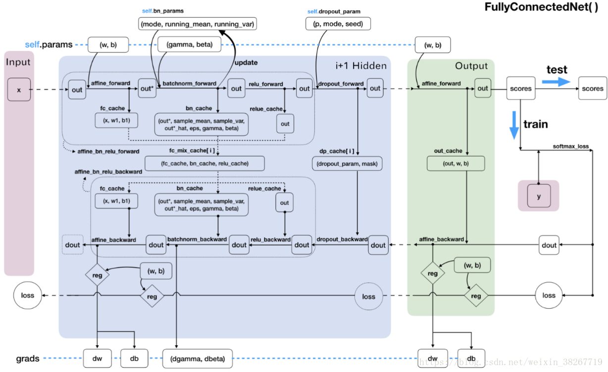
前向传播的线性函数

线性函数。神经网络的层数，3层的神经网络其隐藏层为两层。以三层神经网络为例：h1=x.dot(w1)+b1,h2=h1.dot(w2)+b2，scores=h2.dot(w3)+b3

批量归一化

批量归一化这一步骤在线性函数和激活函数之间，将h1=x.dot(w1)+b1结果拿去激活函数之前进行批量归一化。相当于每一步前向传播都运用了数据预处理的操作，使得加速收敛。

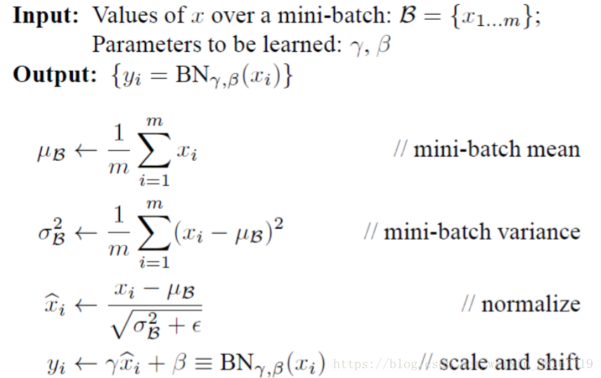
 sample_mean = np.mean(x,axis=0)
 sample_var = np.var(x,axis=0)
 x_hat = (x - sample_mean) / (np.sqrt(sample_var + eps))
 out = gamma * x_hat + beta

这四行代码代表了上面的四个公式，np.mean是求均值，np.var求标准差

正则化

损失函数需要正则化：loss += 0.5 * self.reg * np.sum(self.params["W%d" %(self.num_layers,)]**2)

dw的计算需要正则化：grads["W%d" %(ri+1,)] = dw + self.reg * self.params["W%d" %(ri+1,)]  #每层的dw计算也需要正则化

反向传播

反向传播主要是为了通过最终的得分与其他得分的比较来获得梯度，从而利用梯度更新参数W和b，不断优化权值参数。

以三层神经网络为例：dh2=dscores.dot(w3.T),dw3=h2.T.dot(dscores),db3= np.sum(dscores,axis=0);

dh1=dscores.dot(w2.T),dw2=h1.T.dot(dh2),db2 = np.sum(dh2,axis=0);

dx=dscores.dot(w1.T),dw2=x.T.dot(dh1),db1 = np.sum(dh1,axis=0);

self.params["b%d" %(i+1,)] += -learning_rate * grads["b%d" %(i+1,)]
self.params["W%d" %(i+1,)] += -learning_rate * grads["W%d" %(i+1,)]

数据预处理

PCA是一种预处理形式。在这种处理中，先对数据进行零中心化处理，然后计算协方差矩阵，它展示了数据中的相关性结构。

# 假设输入数据矩阵X的尺寸为[N x D]
X -= np.mean(X, axis = 0) # 对数据进行零中心化(重要)
cov = np.dot(X.T, X) / X.shape[0] # 得到数据的协方差矩阵

数据协方差矩阵的第(i, j)个元素是数据第i个和第j个维度的协方差。具体来说，该矩阵的对角线上的元素是方差。还有，协方差矩阵是对称和半正定的。我们可以对数据协方差矩阵进行SVD（奇异值分解）运算。

U,S,V = np.linalg.svd(cov)

U的列是特征向量，S是装有奇异值的1维数组（因为cov是对称且半正定的，所以S中元素是特征值的平方）。为了去除数据相关性，将已经零中心化处理过的原始数据投影到特征基准上：

Xrot = np.dot(X,U) # 对数据去相关性

U的列是标准正交向量的集合（范式为1，列之间标准正交），所以可以把它们看做标准正交基向量。因此，投影对应x中的数据的一个旋转，旋转产生的结果就是新的特征向量。如果计算Xrot的协方差矩阵，将会看到它是对角对称的。np.linalg.svd的一个良好性质是在它的返回值U中，特征向量是按照特征值的大小排列的。我们可以利用这个性质来对数据降维，只要使用前面的小部分特征向量，丢弃掉那些包含的数据没有方差的维度。 这个操作也被称为主成分分析（ Principal Component Analysis 简称PCA）降维：

Xrot_reduced = np.dot(X, U[:,:100]) # Xrot_reduced 变成 [N x 100]

经过上面的操作，将原始的数据集的大小由[N x D]降到了[N x 100]，留下了数据中包含最大方差的100个维度。通常使用PCA降维过的数据训练线性分类器和神经网络会达到非常好的性能效果，同时还能节省时间和存储器空间。

全过程

http://study.163.com/course/courseLearn.htm?courseId=1003223001&from=study#/learn/text?lessonId=1051303712&courseId=1003223001

一些技巧

超参数更新

采用随机搜索，比如 lr=10**uniform[-6,1)，re=10**uniform[-5,5)，需要注意边界，阶段搜索从粗到细，粗搜索一个周期，然后取决于最佳结果出现在哪里，缩小范围精搜索5个周期。dropout = uniform(0,1)

参数更新

SGD+Nesterov动量

v_prev = v # 存储备份

v = mu * v - learning_rate * dx # 速度更新保持不变

x += -mu * v_prev + (1 + mu) * v # 位置更新变了形式

或者Adam

m = beta1*m + (1-beta1)*dx

v = beta2*v + (1-beta2)*(dx**2)

x += - learning_rate * m / (np.sqrt(v) + eps)

学习率退火

典型的值是每过5个周期就将学习率减少一半，或者每20个周期减少到之前的0.1。或者当验证集错误率停止下降，就乘以一个常数（比如0.5）来降低学习率。

交叉训练

比起交叉验证最好使用一个验证集，在大多数情况下，一个尺寸合理的验证集可以让代码更简单，不需要用几个数据集来交叉验证。

ANN.py

import numpy as np
import matplotlib.pyplot as plt
import math

class TwoLayerNet(object):

  def __init__(self,hidden_dims=[200,100],input_dim=3*32*32+1,num_calsses=10,dropout=0,use_batchnorm=False,reg=0.0,weight_scale=math.sqrt(2/3073),dtype=np.float64,seed=None,std=1e-4):
    self.use_batchnorm = use_batchnorm
    self.use_dropout = dropout>0
    self.reg = reg
    self.num_layers = 1+len(hidden_dims)
    self.dtype = dtype
    self.params = {}
    in_dim = input_dim
    for i,h_dim in enumerate(hidden_dims):  #enumerate的for循环，i对应的是层数，h_dim对应的该层的值
        self.params["W%d" %(i+1,)] = weight_scale * np.random.randn(in_dim,h_dim)  #循环，对每一层W初始化
        self.params["b%d" %(i+1,)] = np.zeros((h_dim,))  #循环，对每一层b初始化
        if use_batchnorm:  #判断是否归一化
            self.params["gamma%d" %(i+1,)] = np.ones((h_dim,))  #初始化每一层的gamma和beta参数
            self.params["beta%d" %(i+1,)] = np.zeros((h_dim,))
        in_dim = h_dim  
    self.params["W%d" %(self.num_layers,)] = weight_scale * np.random.randn(in_dim,num_calsses) #输出层的W和b参数初始化
    self.params["b%d" %(self.num_layers,)] = np.zeros((num_calsses,))
    self.dropout_param = {} 
    if self.use_dropout:   #判断随机失活
        self.dropout_param = {'mode':'train','p':dropout}
    if seed is not None:   #随机失活的种子
        self.dropout_param['seed'] = seed  
    self.bn_params = []
    if self.use_batchnorm:
        self.bn_params = [{'mode':'train'}for i in range(self.num_layers-1)]  #bn_params的前num_layers-1层mode对应的参数是train
    for k,v in self.params.items():
        self.params[k] = v.astype(dtype)
#################################loss损失函数#######################################################################################
  def loss(self, X, y=None):   #损失函数，返回损失值和梯度值
    X = X.astype(self.dtype)   #精度转换
    mode = 'test'if y is None else 'train' #若有y则为train，无y则为test
    if self.dropout_param is not None:
        self.dropout_param['mode'] = mode  
    if self.use_batchnorm:
        for bn_param in self.bn_params:
            bn_param['mode'] = mode
    scores = None
    fc_mix_cache = {}
    if self.use_dropout:
        dp_cache = {}
    out = X
    for i in range(self.num_layers-1):
        w,b = self.params["W%d" %(i+1,)],self.params["b%d" %(i+1,)]
        if self.use_batchnorm:
            gamma = self.params["gamma%d" %(i+1,)]
            beta = self.params["beta%d" %(i+1,)]
            out,fc_mix_cache[i] = self.affine_bn_relu_forward(out,w,b,gamma,beta,self.bn_params[i])
#第一层的返回值是out和fc_mix_cache[1],out为batchnorm和relu激活函数之后的loss，fc_mix_cache返回值是(fc_cache,bn_cache,relu_cache)
#其中fc_cache为计算前的(x,w,b),bn_cache为batchnorm的各个参数，relu_cache为x*w+b之后的h，先x*w+b,再激活,再批量归一化
        else:
            out,fc_mix_cache[i] = self.affine_relu_forward(out,w,b)
        if self.use_dropout:
            out,dp_cache[i] = dropout_forward(out,self.dropout_param)
        
    #最后输出层的w和b
    w = self.params["W%d" %(self.num_layers,)]
    b = self.params["b%d" %(self.num_layers,)]
    out,out_cache = self.affine_forward(out,w,b)
    #out为最终输出的scores,out_cache为隐藏层最后一层的(x,w,b)，若只有一层隐藏层，那就是h1,w2,b2
    scores = out

    if mode == 'test':   #如果是test模式loss函数就只返回scores
        return scores
    loss,grads = 0.0,{}
    #根据最终的scores和y标签的比较，来得到损失值，和dout即dscores=probs=exp_scores / np.sum(exp_scores, axis=1, keepdims=True)
    loss,dout = self.softmax_loss(scores,y)   
    #损失函数正则化
    loss += 0.5 * self.reg * np.sum(self.params["W%d" %(self.num_layers,)]**2)
    dout,dw,db = self.affine_backward(dout,out_cache)#对最后一层，通过dout和(x,w,b)来获得dx,dw,db
    #dw的计算需要进行正则化，db则不需要
    grads["W%d" %(self.num_layers,)] = dw + self.reg * self.params["W%d" %(self.num_layers,)]
    grads["b%d" %(self.num_layers,)] = db

    for i in range(self.num_layers-1): #对所有的隐藏层求dx,dw,db
        ri = self.num_layers-2-i
        #每一层都进行一次损失函数正则化
        loss +=0.5 * self.reg * np.sum(self.params["W%d" %(ri+1,)]**2)
        if self.use_dropout:
            dout = dropout_backward(dout,dp_cache[ri])
        if self.use_batchnorm:  #判断是否进行批量归一化
            #若函数中的dout为dh2，返回的dout为dh1,fc_mix_cache[ri],fc_mix_cache返回值是(fc_cache,bn_cache,relu_cache)
            #其中fc_cache为计算前的(x,w,b)
            dout,dw,db,dgamma,dbeta = self.affine_bn_relu_backward(dout,fc_mix_cache[ri])
            grads["gamma%d" %(ri+1,)] = dgamma
            grads["beta%d" %(ri+1,)] = dbeta
        else:
            dout,dw,db = self.affine_relu_backward(dout,fc_mix_cache[ri])  
            #传是传的fc_mix_cache[ri]=(fc_cache,bn_cache,relu_cache)，用只用fc_cache和relu_cache
        grads["W%d" %(ri+1,)] = dw + self.reg * self.params["W%d" %(ri+1,)]  #每层的dw计算也需要正则化
        grads["b%d" %(ri+1,)] = db
    return loss,grads  #返回的grads包括每层的dw，db，dgamma，dbeta

  def train(self, X, y, X_val, y_val,learning_rate=1e-2, learning_rate_decay=0.95,
            reg=1e-5, num_iters=1000,batch_size=200, verbose=False):
    #batch_size=200，每次迭代抽取200个样本进行损失值和梯度的计算
    num_train = X.shape[0]
    iterations_per_epoch = max(num_train / batch_size, 1)
    loss_history = []
    train_acc_history = []
    val_acc_history = []

    for it in range(num_iters):
      X_batch = None
      y_batch = None
      sample_index = np.random.choice(num_train, batch_size, replace=True)
      X_batch = X[sample_index, :]  # (batch_size,D)
      y_batch = y[sample_index]  # (1,batch_size)
      loss, grads = self.loss(X_batch, y=y_batch)
      loss_history.append(loss) #每次循环所得的loss存在一个loss_history
      ################对参数进行更新##############
      for i in range(self.num_layers-1): #对所有的隐藏层求dx,dw,db
          grads["b%d" %(i+1,)] = grads["b%d" %(i+1,)].reshape(-1)
          self.params["b%d" %(i+1,)] += -learning_rate * grads["b%d" %(i+1,)]
          self.params["W%d" %(i+1,)] += -learning_rate * grads["W%d" %(i+1,)]

      ############################################
      if it % 100 == 0: #循环，每迭代一次就输出一个loss
          print ('iteration %d / %d: loss %f' % (it, num_iters, loss))
      if it % iterations_per_epoch == 0:  #循环结束
        train_acc = (self.predict(X_batch) == y_batch)
        val_acc = (self.predict(X_val) == y_val)
        train_acc_history.append(train_acc)
        val_acc_history.append(val_acc)
        learning_rate *= learning_rate_decay #学习率衰减
    return loss_history

  def predict(self, X):#预测是没有y，则采用test模式
    y_pred = None
    scores = self.loss(X,y_pred)
    y_pred = np.argmax(scores, axis=1)  #返回最高分数的标签list
    return y_pred

  #############################################################前向传播#############################################################
  def affine_bn_relu_forward(self,x,w,b,gamma,beta,bn_param): #先xw+b，再relu，再bathnorm的forward
      a,fc_cache = self.affine_forward(x,w,b)   #xw+b，返回值a=h(i+1)，fc_cache=x,w,b
      a_bn,bn_cache = self.batchnorm_forward(a,gamma,beta,bn_param) #批量归一化，a_bn为归一化后的h
      out,relu_cache = self.relu_forward(a_bn)   #激活函数
      cache = (fc_cache,bn_cache,relu_cache)
      return out,cache
  def affine_relu_forward(self,x,w,b):
       a,fc_cache = self.affine_forward(x,w,b)
       out,relu_cache = self.relu_forward(a)
       cache = (fc_cache,relu_cache)
       return out,cache
  def affine_forward(self,x,w,b):
      out = None
      reshape_x = np.reshape(x,(x.shape[0],-1))
      out = reshape_x.dot(w)+b
      cache = (x,w,b)
      return out,cache

  def relu_forward(self,x):
      out = np.maximum(0,x)
      cache = x
      return out,cache 

    ##############################批量归一化#################################### 
  def batchnorm_forward(self,x,gamma,beta,bn_params):
      mode = bn_params['mode']   #bn_params['mode']
      eps = bn_params.get('eps',1e-5)
      momentum = bn_params.get('momentum',0.9)

      N,D = x.shape
      running_mean = bn_params.get('running_mean',np.zeros(D,dtype=x.dtype))
      running_var = bn_params.get('running_var',np.zeros(D,dtype=x.dtype))

      out,cache = None,None
      if mode == 'train':  #代表1train
          sample_mean = np.mean(x,axis=0)
          sample_var = np.var(x,axis=0)
          x_hat = (x - sample_mean) / (np.sqrt(sample_var + eps))
          out = gamma * x_hat + beta
          cache = (x,sample_mean,sample_var,x_hat,eps,gamma,beta)
          running_mean = momentum * running_mean + (1 - momentum) * sample_mean
          running_var = momentum * running_var + (1 - momentum) * sample_var

      elif mode == 'test': #0代表test
          out = (x - running_mean) * gamma / (np.sqrt(running_var + eps)) + beta
      else:
          raise ValueError('Invaild forward batchnorm mode "%s"' % mode)

      bn_params['running_mean'] = running_mean
      bn_params['running_var'] = running_var
      return out,cache
  ###########################随机失活#############################3
  def dropout_forward(x,dropout_param):
      p,mode = dropout_param['p'],dropout_param['mode']
      if 'seed' in dropout_param:
          np.random.seed(dropout_param['seed'])
      mask = None
      out = None
      
      if mode =='train':
          keep_prob = 1-p
          mask = (np.random.rand(*x.shape)<keep_prob) / keep_prob
          out = mask * x
      elif mode == 'test':
          out = x

      cache = (dropout_param,mask)
      out = out.astype(x.dtype,copy=False)
      return out,cache
  ##################################################################  

  ############################交叉熵损失######################################  
  def softmax_loss(self,z,y):
      scores_max = np.max(z, axis=1, keepdims=True)  # (N,1)
      # Compute the class probabilities
      exp_scores = np.exp(z - scores_max)  # scores - scores_max 那么将f中的值平移到最大值为0,运用的是softmax分类器
      probs = exp_scores / np.sum(exp_scores, axis=1, keepdims=True)  # 按行相加，keepdims=True 并且保持其二维特性
      # cross-entropy loss and L2-regularization
      N = z.shape[0]
      data_loss = -np.sum(np.log(probs[range(N), y])) / N
      dz = probs  # (N,C) 
      dz[range(N), y] -= 1  #  这个是输出的误差敏感项也就是梯度的计算，具体可以看上面softmax 的计算
      dz /= N
      return data_loss,dz
  ##################################################################  

  #############################################################反向传播############################################################  
  def affine_bn_relu_backward(self,dout,cache):
      fc_cache,bn_cache,relu_cache = cache
      da_bn = self.relu_backward(dout,relu_cache)
      da,dgamma,dbeta = self.batchnorm_backward(da_bn,bn_cache)
      dx,dw,db = self.affine_backward(da,fc_cache)
      return dx,dw,db,dgamma,dbeta

  def affine_relu_backward(self,dout,cache):   
      fc_cache,relu_cache = cache
      da = self.relu_backward(dout,relu_cache)
      dx,dw,db = self.affine_backward(da,fc_cache)
      return dx,dw,db 

  def affine_backward(self,dout,cache):  #cache为x,w,b
      z,w,b = cache
      dz,dw,db = None,None,None
      reshaped_x = np.reshape(z,(z.shape[0],-1))
      dz = np.reshape(dout.dot(w.T),z.shape)
      dw = (reshaped_x.T).dot(dout)
      db = np.sum(dout,axis=0)        #dW1 = np.dot(X.T, dh1)  # (D,H)db1 = np.sum(dh1, axis=0, keepdims=True)  # (1,H)
      return dz,dw,db

  def relu_backward(self,dout,cache):  #cache为x
      dx,x = None,cache
      dx = (x >0 ) * dout #与所有x中元素为正的位置处，位置对应于dout矩阵的元素保留，其他都取0
      return dx

  def dropout_backward(dout,cache):
      dropout_param,mask = cache
      mode = dropout_param['mode']

      dx = None
      if mode =='train':
          dx = mask * dout

      elif mode =='test':
          dx = dout
      return dx
#######################批量归一化##############################
  def batchnorm_backward(self,dout,cache):
      x,mean,var,x_hat,eps,gamma,beta = cache
      N = x.shape[0]
      dgamma = np.sum(dout*x_hat,axis=0)
      dbeta = np.sum(dout*1.0,axis=0)
      dx_hat = dout * gamma
      dx_hat_numerator = dx_hat / np.sqrt(var + eps)
      dx_hat_denominator = np.sum(dx_hat * (x - mean),axis=0)
      dx_1 = dx_hat_numerator
      dvar = -0.5 * ((var + eps) ** (-1.5)) * dx_hat_denominator
      dmean = -1.0 * np.sum(dx_hat_numerator,axis=0) + dvar * np.mean(-2.0 * (x-mean),axis=0)
      dx_var =dvar * 2.0 / N * (x - mean)
      dx_mean = dmean * 1.0 / N
      dx = dx_1 + dx_var + dx_mean
      return dx,dgamma,dbeta
##################################################################  

ANNexercise.py

# -*- coding: utf-8 -*-
import pickle as p
import numpy as np
import os


def load_CIFAR_batch(filename):
    """ 载入cifar数据集的一个batch """
    with open(filename, 'rb') as f:
        datadict = p.load(f, encoding='latin1')
        X = datadict['data']
        Y = datadict['labels']
        X = X.reshape(10000, 3, 32, 32).transpose(0, 2, 3, 1).astype("float")
        Y = np.array(Y)
        return X, Y

def load_CIFAR10(ROOT):
    """ 载入cifar全部数据 """
    xs = []
    ys = []
    for b in range(1, 6):
        f = os.path.join(ROOT, 'data_batch_%d' % (b,))
        X, Y = load_CIFAR_batch(f)
        xs.append(X)         #将所有batch整合起来
        ys.append(Y)
    Xtr = np.concatenate(xs) #使变成行向量,最终Xtr的尺寸为(50000,32*32*3)
    Ytr = np.concatenate(ys)
    del X, Y
    Xte, Yte = load_CIFAR_batch(os.path.join(ROOT, 'test_batch'))
    return Xtr, Ytr, Xte, Yte

import numpy as np
import matplotlib.pyplot as plt

# 载入CIFAR-10数据集
cifar10_dir = 'datasets/cifar-10-batches-py'
X_train, y_train, X_test, y_test = load_CIFAR10(cifar10_dir)


# 看看数据集中的一些样本：每个类别展示一些
print('Training data shape: ', X_train.shape)
print('Training labels shape: ', y_train.shape)
print('Test data shape: ', X_test.shape)
print('Test labels shape: ', y_test.shape)

num_train=40000
num_validation=5000
num_test=5000
num_dev=500

mask=range(num_train,num_train+num_validation)
X_val=X_train[mask]
y_val=y_train[mask]

mask=range(num_train)
X_train=X_train[mask]
y_train=y_train[mask]

mask=np.random.choice(num_train,num_dev,replace=False)
X_dev=X_train[mask]
y_dev=y_train[mask]

mask=range(num_test)
X_test=X_test[mask]
y_test=y_test[mask]

X_train=np.reshape(X_train,(X_train.shape[0],-1))
X_dev=np.reshape(X_dev,(X_dev.shape[0],-1))
X_val=np.reshape(X_val,(X_val.shape[0],-1))
X_test=np.reshape(X_test,(X_test.shape[0],-1))


print('Training data shape: ', X_train.shape)
print('Training labels shape: ', y_train.shape)
print('Test data shape: ', X_test.shape)
print('Test labels shape: ', y_test.shape)

#首先训练数据，计算图像的平均值
mean_image=np.mean(X_train,axis=0)#计算每一列特征的平均值，共32*32*3个特征
print(mean_image[:10])  #查看指定特征的数据
plt.figure(figsize=(4,4))  #指定画框框图的大小 
plt.imshow(mean_image.reshape((32,32,3)).astype('uint8'))  #将平均值可视化
#plt.show()


X_train-=mean_image  #去中心化
X_dev-=mean_image
X_test-=mean_image
X_val-=mean_image

X_train=np.hstack([X_train,np.ones((X_train.shape[0],1))])  #多出了包含常量1的1个维度
X_dev=np.hstack([X_dev,np.ones((X_dev.shape[0],1))])
X_test=np.hstack([X_test,np.ones((X_test.shape[0],1))])
X_val=np.hstack([X_val,np.ones((X_val.shape[0],1))])


import ANN

learning_rates=[1e-2]
regularization_strengths = [0.6]
results={}
best_val=-1
best_ann = None

for rate in learning_rates:
    for regular in regularization_strengths:
        ann=ANN.TwoLayerNet()
        loss_history=ann.train(X_train, y_train, X_val, y_val,learning_rate=rate, learning_rate_decay=0.95,reg=regular, num_iters=1000,batch_size=2000, verbose=False)
        y_train_pred=ann.predict(X_train)
        accuracy_train = np.mean(y_train==y_train_pred)
        y_val_pred=ann.predict(X_val)
        accuracy_val = np.mean(y_val==y_val_pred)
        results[(rate,regular)] = (accuracy_train,accuracy_val)
        if (best_val < accuracy_val):
            best_val = accuracy_val
            best_ann = ann
for lr,reg in sorted(results):
    train_accuracy,val_accuracy = results[(lr,reg)]
    print('lr %e reg %e train accuracy: %f val accracy: %f'%(lr,reg,train_accuracy,val_accuracy))
print('best_val_accuracy: %f'%(best_val))
y_tset_pred = best_ann.predict(X_test)
acc_test = np.mean(y_test == y_tset_pred)
print('test_accuracy: %f'%(acc_test))