python深度学习进阶（自然语言处理）-自然语言和单词的分布式表示

最新推荐文章于 2024-01-25 10:04:00 发布

诗雨时

最新推荐文章于 2024-01-25 10:04:00 发布

阅读量2.8k

点赞数 5

分类专栏：人工智能（深度学习进阶）

本文链接：https://blog.csdn.net/weixin_38477351/article/details/116427487

版权

人工智能（深度学习进阶）专栏收录该内容

2 篇文章 2 订阅

订阅专栏

深度学习进阶（自然语言处理）-自然语言和单词的分布式表示

博主微信公众号（左）、Python+智能大数据+AI学习交流群（右）：欢迎关注和加群，大家一起学习交流，共同进步！

3.1 基于 Python 的语料库的预处理

摘要

使用 WordNet 等同义词词典，可以获取近义词或测量单词间的相似度等。
使用同义词词典的方法存在创建词库需要大量人力、新词难更新等问题。
目前，使用语料库对单词进行向量化是主流方法。
近年来的单词向量化方法大多基于 “单词含义由其周围的单词构成” 这一分布式假设。
在基于计数的方法中，对语料库中的每个单词周围的单词的出现频数进行计数并汇总（=共现矩阵）。
通过将共现矩阵转化为 PPMI 矩阵并降维，可以将大的稀疏向量转变为小的密集向量。
在单词的向量空间中，含义上接近的单词距离上理应也更近。

1. 什么是自然语言处理

自然语言（natural language）：我们平常使用的语言，如汉语或英语，称为自然语言（natural language）。

自然语言处理（Natural Language Processing，NLP）：顾名思义，就是处理自然语言的科学。简单地说，它是一种能够让计算机理解人类语言的技术。换言之，自然与处理的目标就是让计算机理解人说的话，进而完成对我们有帮助的事情。

我们的语言是由文字构成的，而语言的含义是由单词构成的。换句话说，单词是含义的最小单位。

2. 同义词词典

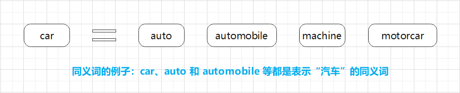
同义词词典（thesaurus）：具有相同含义的单词（同义词）或含义类似的单词（近义词）被归类到同一个组中。比如，使用同义词词典，我们可以知道 car 的同义词有 automobile、motorcar等（图 2-1）。

在自然语言处理中用到的同义词词典有时会定义比单词之间的粒度更细的关系，比如 “上位-下位” 关系、“整体-部分” 关系。举个例子，如图 2-2 所示，我们利用图结构定义了各个单词之间的关系。

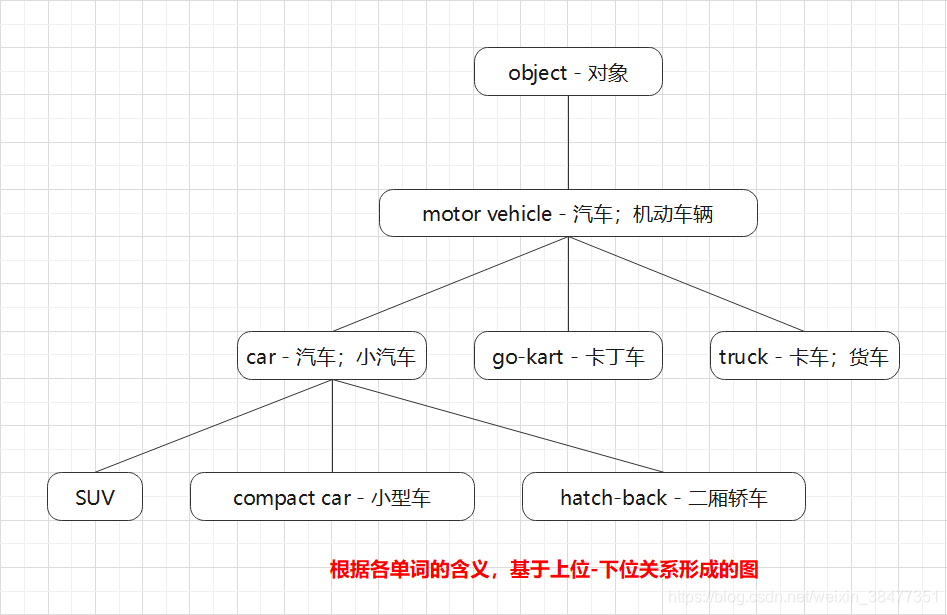
在图 2-2 中，单词 motor vehicle（机动车）是单词 car 的上位概念。car 的下位概念有 SUV、compact car 和 hatch-back 等更加具体的车种。

像这样，通过对所有单词创建近义词集合，并用图表示各个单词的关系，可以定义单词之间的联系。利用这个 “单词网络”，可以教会计算机单词之间的相关性。也就是说，我们可以将单词含义（间接地）教给计算机，然后利用这一知识，就能让计算机做一些对我们有用的事情。

如何使用同义词词典根据自然语言处理的具体应用的不同而不同。比如，在信息检索场景中，如果事先知道 automobile 和 car 是近义词，就可以将 automobile 的检索结果添加到 car 的检索结果中。

2.1 WordNet

WordNet：自然语言处理领域最著名的同义词词典。由普林斯顿大学于 1985 年开始开发的同义词词典。

使用 WordNet，可以获得单词的近义词，或者利用单词网络。使用单词网络，可以计算单词之间的相似度。

2.2 同义词词典的问题

难以顺应时代变化

我们使用的语言是活的。随着时间的推移，新词不断出现，而那些落满尘埃的旧词不知哪天就会被遗忘。比如，“众筹”（crowdfunding）就是一个最近才开始使用的新词。

另外，语言的含义也会随着时间的推移而变化。比如，英语中的 heavy 一词，现在有 “事态严重” 的含义（主要用于俚语），但以前是没有这种用法的。在电影《回到未来》中，有这样一个场景：从 1985 年穿越回来的马蒂和生活在 1955 年的博士的对话中，对 heavy 的含义有不同的理解。如果要处理这样的单词变化，就需要人工不停地更新同义词词典。

人力成本高

制作词典需要巨大的人力成本。以英文为例，据说现有的英文单词总数超过 1000 万个。在极端情况下，还需要对如此大规模的单词进行单词之间的关联。

顺便提一下，WordNet 中收录了超过 20 万个的单词。

无法表示单词的微妙关系

同义词词典中将含义相近的词分到一组。但实际上，即使含义相近的单词，也有细微的差别。比如，wintage(复古) 和 retro(复古)虽然表示相同的含义，但是用法不同，而这种细微的差别在同义词词典中是无法表示出来的。

3. 基于计数的方法

语料库（corpus）：大量的文本数据。语料库中包含了大量的关于自然语言的实践知识，即文章的写作方法、单词的选择方法和单词含义等。

3.1 基于 Python 的语料库的预处理

import re
import numpy as np


def preprocess(text):
    """
    文本语料预处理
    :param text: 需要进行预处理的文本内容
    :return:
    """
    text = text.lower()    # 将所有字母转化为小写

    # 方案一
    words = re.split("\W+", text)    # \W 匹配任何非单词字符。等价于 "[^A-Za-z0-9_]"

    # 方案二
    # text = text.replace(".", " .")    # 句尾的句号前插入一个空格
    # words = text.split(" ")    # 通过空格分割句子

    word_to_id = {}    # 将单词转化为单词ID（健是单词，值是单词ID）
    id_to_word = {}    # 将单词ID转化为单词（健是单词ID，值是单词）
    for word in words:
        if word not in word_to_id:
            new_id = len(word_to_id)
            word_to_id[word] = new_id
            id_to_word[new_id] = word

    # 单词列表转化为单词ID列表
    corpus = np.array([word_to_id[w] for w in words])

    return corpus, word_to_id, id_to_word


if __name__ == "__main__":
    text = "You say goodbye and I say hello."
    corpus, word_to_id, id_to_word = preprocess(text)
    print(corpus)
    print(word_to_id)
    print(id_to_word)

[0 1 2 3 4 1 5 6]
{'you': 0, 'say': 1, 'goodbye': 2, 'and': 3, 'i': 4, 'hello': 5, '': 6}
{0: 'you', 1: 'say', 2: 'goodbye', 3: 'and', 4: 'i', 5: 'hello', 6: ''}

3.2 单词的分布式表示

单词的分布式表示：将单词表示为固定长度的向量。

这种向量的特征在于它是用密集向量表示的。密集向量的意思是，向量的各个元素（大多数）是由非 0 实数表示的。例如，三维分布表示是 [0.21, -0.45, 0.83]。

3.3 分布式假设

分布式假设（distributional hypothesis）：某个单词的含义由它周围的单词形成。

单词本身没有含义，单词含义由它所在的上下文（语境）形成。的确，含义相同的单词经常出现在相同的语境中。比如 “I drink beer.” “I drink wine.”，drink 的附近常有饮料出现。另外，从 “I guzzle beer.” “I guzzle wine.” 可知，guzzle(大口喝) 和 drink(喝) 所在的语境相同。进而我们可以推测出，guzzle 和 drink 是近义词。

上下文：某个居中单词（关注词）周围的单词（词汇）。在图 2-3 的例子中，左侧和右侧的 2 个单词就是上下文。

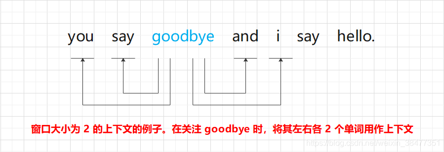
将左右两边相同数量的单词作为上下文。但是，根据具体情况，也可以仅将左边的单词或者右边的单词作为上下文。此外，也可以使用考虑了句子分隔符的上下文。

窗口大小（window size）：将上下文的大小（即周围的单词有多少个）称为窗口大小（window size）。

窗口大小为 1，上下文包含左右各 1个单词；窗口大小为 2，上下文包含左右各 2 个单词，以此类推。

3.4 共现矩阵

基于计数的方法：在关注某个单词的情况下，对它的周围出现了多少次什么单词进行计数，然后汇总（根据一个单词周围的单词的出现频数来表示该单词）。

计算 “you say goodbye and i say hello.” 中各个单词的上下文中包含的单词的频数：

设置窗口大小为 1，从单词 ID 为 0 的 you 开始。

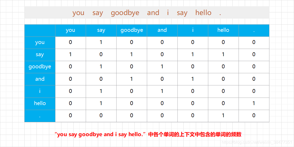
图 2-4 “you say goodbye and i say hello.”中各个单词的上下文中包含的单词的频数

图 2-4 是汇总了所有单词的共现单词的表格。这个表格的各行对应相应单词的向量。因为图 2-4 的表格呈矩阵状，所以称为共现矩阵（co-occurence matrix）。

def create_co_matrix(corpus, vocab_size, window_size=1):
    """
    生成共现矩阵
    :param corpus: 语料库（单词ID列表）
    :param vocab_size: 词汇个数
    :param window_size: 窗口大小（当窗口大小为1时，左右各1个单词为上下文）
    :return: 共现矩阵
    """
    corpus_size = len(corpus)
    co_matrix = np.zeros((vocab_size, vocab_size), dtype=np.int32)

    for idx, word_id in enumerate(corpus):
        for i in range(1, window_size + 1):
            left_idx = idx - i
            right_idx = idx + i

            if left_idx >= 0:
                left_word_id = corpus[left_idx]
                co_matrix[word_id, left_word_id] += 1

            if right_idx < corpus_size:
                right_word_id = corpus[right_idx]
                co_matrix[word_id, right_word_id] += 1

    return co_matrix

3.5 向量间的相似度

测量单词的向量表示的相似度的方法：余弦相似度（cosine similarity）。设有 $x = (x_{1}, x_{2}, x_{3}, ... , x_{n})$ 和 $y=({y_{1}, y_{2}, y_{3}, ... , y_{n}})$ 两个向量，它们之间的余弦相似度的定义方式如下式所示。

$similarity(x, y) = \frac{x\cdot y}{\left \|x \left \| \right \| y\right \|}=\frac{x_{1}y_{1}+ ... + x_{n}y_{n}}{\sqrt{x_{1}^{2}+ ... + x_{n}^{2}}\sqrt{y_{1}^{2}+ ... + y_{n}^{2}}} \ \ \ \ \ \ \ \ (2.1)$

式 (2.1) 中，分子是向量内积，分母是各个向量的范数。范数表示向量的大小，这里计算的是 $L2$ 范数（即向量各个元素的平方和的平方根）。式 (2.1) 的要点是先对向量进行正规化，再求它们的内积。

余弦相似度直观地表示了 “两个向量在多大程度上指向同一方向”。两个向量完全指向相同的方向时，余弦相似度为 1；完全指向相反的方向时，余弦相似度为 -1。

Python 实现余弦相似度计算：

def cos_similarity(x, y, eps=1e-8):
    """
    计算余弦相似度
    :param x: 向量
    :param y: 向量
    :param eps: 用于防止“除数为0”的微小值
    :return:
    """
    nx = x / (np.sqrt(np.sum(x ** 2)) + eps)    # x的正规化
    ny = y / (np.sqrt(np.sum(y ** 2)) + eps)    # y的正规化

    return np.dot(nx, ny)    # 计算两个向量的内积

实验：求句子 "You say goodbye and I say hello." 中单词 "You" 和单词 "I" 的相似度。

"""余弦相似度"""

import sys

sys.path.append("..")
from common.util import preprocess, create_co_matrix, cos_similarity

text = "You say goodbye and I say hello."    # 文本
corpus, word_to_id, id_to_word = preprocess(text)    # 文本语料预处理
vocab_size = len(word_to_id)    # 词汇大小
matrix = create_co_matrix(corpus, vocab_size)    # 生成共现矩阵

vector_you = matrix[word_to_id["you"]]    # you的单词向量
vector_i = matrix[word_to_id["i"]]        # i的单词向量

con_simi = cos_similarity(vector_you, vector_i)    # 计算余弦相似度
print(con_simi)

# 0.7071067691154799

从上面的结果可知，"you" 和 "i" 的余弦相似度是 0.7071067691154799。由于余弦相似度的取值范围是 -1 到 1，所以可以说这个值是相对较高的（存下相似性）。

3.6 相似单词的排序

实验：当某个单词被作为查询词时，将与这个查询词相似的单词按降序显示出来。

def most_similarity(query, word_to_id, id_to_word, word_matrix, top=5):
    """
    相似单词的查找
    :param query: 查询词
    :param word_to_id: 从单词到单词ID的字典
    :param id_to_word: 从单词ID到单词的字典
    :param word_matrix: 汇总了单词向量的矩阵，假定保存了与各行对应的单词向量
    :param top: 显示到前几位
    :return:
    """
    # 1. 取出查询词的单词向量
    if query not in word_to_id:
        print(f"{query} is not found")
        return

    print(f"\n[query]{query}")
    query_id = word_to_id[query]
    query_vector = word_matrix[query_id]

    # 2. 分别求得查询词的单词向量和其他所有单词向量的余弦相似度
    vocab_size = len(word_to_id)    # 词汇大小
    similarity = np.zeros(vocab_size)
    for i in range(vocab_size):
        similarity[i] = cos_similarity(word_matrix[i], query_vector)

    # 3. 基于余弦相似度的结果，按降序显示它们的值
    count = 0
    for i in (-1 * similarity).argsort():
        if id_to_word[i] == query:
            continue
        print(f"{id_to_word[i]}: {similarity[i]}")

        count += 1
        if count >= top:
            return

"""当某个单词被作为查询词时，将与这个查询词相似的单词按降序显示出来"""

import sys

sys.path.append("..")
from common.util import preprocess, create_co_matrix, most_similarity

text = "You say goodbye and I say hello."    # 文本
corpus, word_to_id, id_to_word = preprocess(text)    # 文本语料预处理
vocab_size = len(word_to_id)    # 词汇大小
matrix = create_co_matrix(corpus, vocab_size)    # 生成共现矩阵

# 将与单词"you"相似的单词按降序显示出来
most_similarity("you", word_to_id, id_to_word, matrix, top=5)

[query]you
goodbye: 0.7071067691154799
i: 0.7071067691154799
hello: 0.7071067691154799
say: 0.0
and: 0.0

4. 基于计数的方法的改进

4.1 点互信息

针对高频词汇（出现次数很多的单词），根据共现矩阵统计两个单词同时出现的次数，可能会存在相关性误差。比如：我们来考虑某个语料库中 the 和 car 共现的情况。

在这种情况下，我们会看到很多 “...the car...” 这样的短语。因此，它们的共现次数将会很大。另外，car 和 drive 也明显有很强的相关性。但是，如果只看单词的出现次数，那么与 drive 相比，the 和 car 的相关性更强。这意味着，仅仅因为 the 是个常用词，它就被认为与 car 有很强的相关性。

点互信息（Pointwise Mutual Information，PMI）：对于随机变量 $x$ 和 $y$ ，它们的 PMI 定义如下：

$PMI(x, y) = \frac{P(x, y)}{P(x)P(y)} \ \ \ \ \ \ \ \ (2.2)$

   $P(x)$ ：单词 $x$ 在语料库中出现的概率。

   $P(y)$ ：单词 $y$ 在语料库中出现的概率。

   $P(x,y)$ ：单词 $x$ 和 $y$ 同时在语料库中出现的概率。

注：PMI 的值越高，表明相关性越强。

PMI 示例：假设某个语料库中有 10000 个单词，其中单词 the 出现了 100 次，单词 the 和 car 同时出现了 10 次，分别计算 P("the") 和 P("the", "car")。

$P("the") = \frac{100}{10000} = 0.01 \ \ \ \ P("the", "car") = \frac{10}{10000} = 0.001$

使用共现矩阵（其元素表示单词共现的次数）重写式 (2.2)，根据共现矩阵求 PMI：

$PMI(x, y) = log_{2}\frac{\frac{C(x, y)}{N}}{\frac{C(x)}{N}\frac{C(y)}{N}} = log_{2}\frac{C(x, y) \cdot N}{C(x)C(y)} \ \ \ \ \ \ \ \ (2.3)$

$C$ ：共现矩阵。

   $C(x, y)$ ：单词 $x$ 和 $y$ 的共现次数。

   $C(x)$ ：单词 $x$ 的出现次数。

   $C(y)$ ：单词 $y$ 的出现次数。

根据共现矩阵求 PMI 示例：假设语料库中的单词数量（N）为 10000，the 出现 1000 次，car 出现 20 次，drive 出现 10 次，the 和 car 共现 10 次，car 和 drive 共现 5 次。

$PMI("the", "car") = log_{2}\frac{10 \cdot 10000}{1000 \cdot 20} \approx 2.32$

$PMI("car", "drive") = log_{2}\frac{5 \cdot 10000}{20 \cdot 10} \approx 7.97$

PMI 存在的问题：当两个单词的共现次数为 0 时， $log_{2}0=-\infty$ 。

正的点互信息（Positive PMI，PPMI）：

$PPMI(x, y) = max(0, PMI(x, y)) \ \ \ \ \ \ \ \ (2.4)$

当 PMI 是负数时，将其视为 0，这就可以将单词间的相关性表示为大于 0 的实数。

使用 Python 实现将共现矩阵转化为 PPMI 矩阵：

当单词 $x$ 和单词 $y$ 的共现次数为 $C(x, y)$ 时， $C(x) = \sum_{i}C(i, x)$ ， $C(y) = \sum_{i}C(i, y)$ ， $C(x, y) = \sum_{i}\sum_{j}C(i, j)$ ，进行这样的近似并实现。

def ppmi(C, verbose=False, eps=1e-8):
    """
    生成PPMI（正的点互信息）
    :param C: 共现矩阵
    :param verbose: 是否输出运行情况
    :param eps: 用于防止对数运算发散到负无穷大的微小值
    :return:
    """
    M = np.zeros_like(C, dtype=np.float32)
    N = np.sum(C)
    S = np.sum(C, axis=0)
    total = C.shape[0] * C.shape[1]
    cnt = 0

    for i in range(C.shape[0]):
        for j in range(C.shape[1]):
            pmi = np.log2(C[i, j] * N / (S[j] * S[i]) + eps)
            M[i, j] = max(0, pmi)

            if verbose:
                cnt += 1
                if cnt % (total // 100+1) == 0:
                    print("%.1f%% done" % (100 * cnt / total))
    return M

"""讲共现矩阵转化为PPMI矩阵"""

import sys
import numpy as np
sys.path.append("..")

from common.util import preprocess, create_co_matrix, cos_similarity, ppmi

text = "You say goodbye and I say hello."   # 文本
corpus, word_to_id, id_to_word = preprocess(text)   # 文本语料预处理
vocab_size = len(word_to_id)    # 词汇大小

C = create_co_matrix(corpus, vocab_size)    # 生成共现矩阵
W = ppmi(C)     # 讲共现矩阵转化为 PPMI 矩阵

np.set_printoptions(precision=3)    # 有效位数为3位
print("covariance matrix")
print(C)
print("-" * 50)
print("PPMI")
print(W)

covariance matrix
[[0 1 0 0 0 0 0]
 [1 0 1 0 1 1 0]
 [0 1 0 1 0 0 0]
 [0 0 1 0 1 0 0]
 [0 1 0 1 0 0 0]
 [0 1 0 0 0 0 1]
 [0 0 0 0 0 1 0]]
--------------------------------------------------
PPMI
[[0.    1.807 0.    0.    0.    0.    0.   ]
 [1.807 0.    0.807 0.    0.807 0.807 0.   ]
 [0.    0.807 0.    1.807 0.    0.    0.   ]
 [0.    0.    1.807 0.    1.807 0.    0.   ]
 [0.    0.807 0.    1.807 0.    0.    0.   ]
 [0.    0.807 0.    0.    0.    0.    2.807]
 [0.    0.    0.    0.    0.    2.807 0.   ]]

PPMI 矩阵的各个元素均为大于等于 0 的实数。我们得到了一个由更好的指标形成的矩阵，这相当于获取了一个更好的单词向量。

PPMI 存在的问题：

(1) 随着语料库的词汇量增加，各个单词向量的维数也会增加。（如果语料库的词汇达到 10 万，则单词向量的维数也同样会达到 1 0 万。）

(2) PPMI 矩阵中很多元素都是 0。这表明向量中的绝大多数元素并不重要，也就是说，每个元素拥有的 “重要性” 很低。

(3) PPMI 矩阵中的歌单词向量容易受到噪声的影响，稳健性差。

注意：可以使用向量降维的方法，解决 PPMI 存在的这些问题。

4.2 降维

降维（dimensionality reduction）：减少向量的维度（在尽量保留 “重要信息” 的基础上减少）。

稀疏矩阵（稀疏向量）：向量中的大多数元素为 0 的矩阵（或向量）称为稀疏矩阵（或稀疏向量）。

这里的重点是，从稀疏矩阵中找出重要的轴，用更少的维度对其进行重新表示。结果，稀疏矩阵就会被转化为大多数元素均不为 0 的秘籍矩阵。这个密集矩阵就是我们想要的单词的分布式表示。

奇异值分解（Singular Value Decomposition，SVD）：一种降维的方法。将任意的矩阵分解为 3 个矩阵的乘积，如下式所示：

$X=USV^{T} \ \ \ \ \ \ \ \ (2.5)$

SVD 将任意的矩阵 X 分解为 U、S、V 这 3 个矩阵的乘积，其中 U 和 V 是列向量彼此正交的正交矩阵，S 是除了对角线元素以外其余元素均为 0 的对角矩阵。

4.3 基于 SVD 的降维

"""基于SVD的降维"""

import sys
sys.path.append("..")

import numpy as np
from matplotlib import pyplot as plt

from common.util import preprocess, create_co_matrix, ppmi

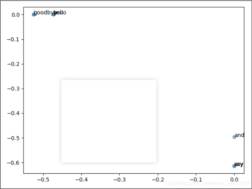
text = "You say goodbye and I asy hello"
corpus, word_to_id, id_to_word = preprocess(text)
vocab_size = len(id_to_word)
C = create_co_matrix(corpus, vocab_size, window_size=1)
W = ppmi(C)

# SVD
U, S, V = np.linalg.svd(W)

# 查看单词ID为0的单词向量
print(C[0])    # 共现矩阵
print(W[0])    # PPMI矩阵
print(U[0])    # SVD

# plot
for word, word_id in word_to_id.items():
    plt.annotate(word, (U[word_id, 0], U[word_id, 1]))    # 在2D图形中坐标为(x, y)的地方绘制单词的文本

plt.scatter(U[:, 0], U[:, 1], alpha=0.5)    # 绘制散点图
plt.show()

图 2-5 对共现矩阵执行SVD，并在图上绘制各个单词的二维向量（i 和 goodbye 重叠）

4.4 PTB 数据集

"""Penn Treebank 语料库数据集下载"""
import os
import sys
sys.path.append("..")

try:
    import urllib.request
except ImportError:
    raise ImportError("Please Use Python3!")
import pickle
import numpy as np

url_base = "https://raw.githubusercontent.com/tomsercu/lstm/master/data/"
key_file = {
    "train": "ptb.train.txt",
    "test": "ptb.test.txt",
    "valid": "ptb.valid.txt"
}
save_file = {
    "train": "ptb.train.npy",
    "test": "ptb.test.npy",
    "valid": "ptb.valid.npy"
}
vocab_file = "ptb.vocab.pkl"

dataset_dir = os.path.dirname(os.path.abspath(__file__))


def _download(file_name):
    """下载数据"""
    file_path = dataset_dir + "/" + file_name
    if os.path.exists(file_path):
        return

    print("Downloading " + file_name + " ... ")

    try:
        urllib.request.urlretrieve(url_base + file_name, file_path)
    except urllib.error.URLError:
        import ssl
        ssl._create_default_https_context = ssl._create_unverified_context
        urllib.request.urlretrieve(url_base + file_name, file_path)

    print("Done")


def load_vocab():
    """加载词向量"""
    vocab_path = dataset_dir + "/" + vocab_file

    if os.path.exists(vocab_path):
        with open(vocab_path, "rb") as f:
            word_to_id, id_to_word = pickle.load(f)
        return word_to_id, id_to_word

    word_to_id, id_to_word = {}, {}
    data_type = "train"
    file_name = key_file[data_type]
    file_path = dataset_dir + "/" + file_name

    _download(file_name)

    words = open(file_path).read().replace("\n", "<eos>").strip().split()

    for i, word in enumerate(words):
        if word in word_to_id:
            continue
        tmp_id = len(word_to_id)
        word_to_id[word] = tmp_id
        id_to_word[tmp_id] = word

    with open(vocab_path, "wb") as f:
        pickle.dump((word_to_id, id_to_word), f)

    return word_to_id, id_to_word


def load_data(data_type="train"):
    """
    加载数据
    :param data_type: 数据的种类："train" or "test" or "valid(val)"
    :return:
    """
    if data_type == "val": data_type = "valid"
    save_path = dataset_dir + "/" + save_file[data_type]

    word_to_id, id_to_word = load_vocab()

    if os.path.exists(save_path):
        corpus = np.load(save_path)
        return corpus, word_to_id, id_to_word

    file_name = key_file[data_type]
    file_path = dataset_dir + "/" + file_name
    _download(file_name)

    words = open(file_path).read().replace("\n", "<eos>").strip().split()
    corpus = np.array([word_to_id[w] for w in words])

    np.save(save_path, corpus)
    return corpus, word_to_id, id_to_word


if __name__ == "__main__":
    for data_type in ("train", "val", "test"):
        load_data(data_type)

"""获取Penn Treebank数据集"""

import sys
sys.path.append("..")

from dataset import ptb

corpus, word_to_id, id_to_word = ptb.load_data("train")

print(f"corpus size: {len(corpus)}")
print(f"corpus[:30]: {corpus[:30]}")
print()

print(f"id_to_word[0]: {id_to_word[0]}")
print(f"id_to_word[1]: {id_to_word[1]}")
print(f"id_to_word[2]: {id_to_word[2]}")
print()

print(f"word_to_id['car']: {word_to_id['car']}")
print(f"word_to_id['happy']: {word_to_id['happy']}")
print(f"word_to_id['lexus']: {word_to_id['lexus']}")

corpus size: 929589
corpus[:30]: [ 0  1  2  3  4  5  6  7  8  9 10 11 12 13 14 15 16 17 18 19 20 21 22 23
 24 25 26 27 28 29]

id_to_word[0]: aer
id_to_word[1]: banknote
id_to_word[2]: berlitz

word_to_id['car']: 3856
word_to_id['happy']: 4428
word_to_id['lexus']: 7426

corpus：保存了单词 ID 列表；

id_to_word：将单词 ID 转化为单词的字典；

word_to_id：将单词转化为单词 ID 的字典。

4.3 基于 PTB 数据集的评价

实验：将使用快速的SVD进行降维，将基于计数的方法应用于PTB数据集。

"""将使用快速的SVD进行降维，将基于计数的方法应用于PTB数据集"""

import sys
sys.path.append("..")
import numpy as np

from dataset import ptb
from common.util import most_similarity, create_co_matrix, ppmi

window_size = 2
wordvec_size = 100

corpus, word_to_id, id_to_word = ptb.load_data("train")
vocab_size = len(word_to_id)
print("counting co-occurrence ...")
C = create_co_matrix(corpus, vocab_size, window_size)
print("calculating PPMI ...")
W = ppmi(C, verbose=True)

print("calculating SVD ...")
try:
    # truncated SVD (fast!)
    from sklearn.utils.extmath import randomized_svd
    U, S, V = randomized_svd(W, n_components=wordvec_size, n_iter=5, random_state=None)
except ImportError:
    # SVD
    U, S, V = np.linalg.svd(W)

word_vecs = U[:, :wordvec_size]

querys = ["you", "year", "car", "toyota"]
for query in querys:
    most_similarity(query, word_to_id, id_to_word, word_vecs, top=5)

[query]you
we: 0.6613374948501587
i: 0.6418123245239258
'll: 0.5933582186698914
do: 0.5657934546470642
else: 0.542672872543335

[query]year
next: 0.6690017580986023
quarter: 0.6489037871360779
month: 0.6386873722076416
earlier: 0.638314425945282
third: 0.6009232401847839

[query]car
auto: 0.59914231300354
luxury: 0.522028923034668
corsica: 0.5101985931396484
domestic: 0.49824029207229614
truck: 0.46317732334136963

[query]toyota
motor: 0.7657813429832458
nissan: 0.6762233972549438
motors: 0.6223803162574768
honda: 0.6207777261734009
lexus: 0.6151211261749268

对于查询词 you：i、we 等人称代词排在前面，这些都是在语法上具有相同用法的词。

对于查询词 year：next、quarter、month 等近义词。

对于查询词 car：auto、luxury 等近义词。

对于查询词 toyoto：出现了 nisson、honda、lexus 等汽车制造商名或者品牌名。