


获取案例链接、直播课件、数据集在本公众号内发送“机器学习”。
机器学习模型的求解最终都会归结为求解一个最优化问题,最优化的目标为模型误差,它是模型参数的函数。例如线性回归的优化目标是均方误差,参数是每个特征的系数。根据目标函数的特点(凸与非凸),样本数量,特征数量,在实践中会选择不同的优化方法。常见的优化方法包括解析法、梯度下降法、共轭梯度法、交替迭代法等。本案例将对常见的优化算法进行分析,以便理解不同优化方法的特点和适用场景,帮助我们在机器学习实践中选择最合适的优化方法。
1 Python 梯度下降法实现
import matplotlib.pyplot as plt
import numpy as np

from mpl_toolkits.mplot3d import Axes3D
from matplotlib import animation
from IPython.display import HTML

from autograd import elementwise_grad, value_and_grad,grad
from scipy.optimize import minimize
from scipy import optimize
from collections import defaultdict
from itertools import zip_longest
plt.rcParams['axes.unicode_minus']=False  # 用来正常显示负号
1.1 实现简单优化函数
借助 Python 的匿名函数定义目标函数。
f1 = lambda x1,x2 : x1**2 + 0.5*x2**2 #函数定义
f1_grad = value_and_grad(lambda args : f1(*args)) #函数梯度
1.2 梯度下降法实现
梯度下降法使用以下迭代公式进行参数的更新。
其中 为学习率。我们实现 gradient_descent 方法来进行参数的更新。
def gradient_descent(func, func_grad, x0, learning_rate=0.1, max_iteration=20):
    path_list = [x0]
    best_x = x0
    step = 0
    while step         update = -learning_rate * np.array(func_grad(best_x)[1])
        if(np.linalg.norm(update) 1e-4):
            break
        best_x = best_x + update
        path_list.append(best_x)
        step = step + 1
    return best_x, np.array(path_list)
2 梯度下降法求解路径可视化
首先我们使用上节实现的梯度下降法求解,得到参数的优化路径。
best_x_gd, path_list_gd = gradient_descent(f1,f1_grad,[-4.0,4.0],0.1,30)
path_list_gd
array([[-4. , 4. ],
[-3.2 , 3.6 ],
[-2.56 , 3.24 ],
[-2.048 , 2.916 ],
[-1.6384 , 2.6244 ],
[-1.31072 , 2.36196 ],
[-1.048576 , 2.125764 ],
[-0.8388608 , 1.9131876 ],
[-0.67108864, 1.72186884],
[-0.53687091, 1.54968196],
[-0.42949673, 1.39471376],
[-0.34359738, 1.25524238],
[-0.27487791, 1.12971815],
[-0.21990233, 1.01674633],
[-0.17592186, 0.9150717 ],
[-0.14073749, 0.82356453],
[-0.11258999, 0.74120808],
[-0.09007199, 0.66708727],
[-0.07205759, 0.60037854],
[-0.05764608, 0.54034069],
[-0.04611686, 0.48630662],
[-0.03689349, 0.43767596],
[-0.02951479, 0.39390836],
[-0.02361183, 0.35451752],
[-0.01888947, 0.31906577],
[-0.01511157, 0.2871592 ],
[-0.01208926, 0.25844328],
[-0.00967141, 0.23259895],
[-0.00773713, 0.20933905],
[-0.0061897 , 0.18840515],
[-0.00495176, 0.16956463]])
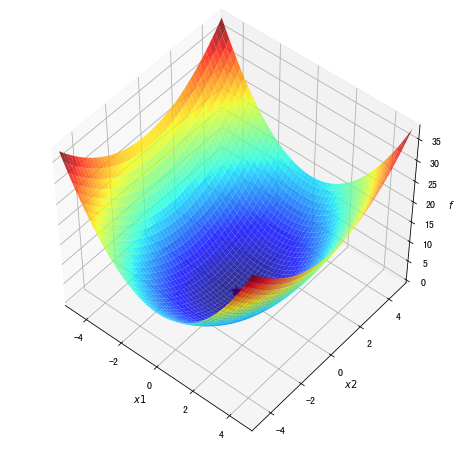
2.1 目标函数曲面的可视化
为了将函数曲面绘制出来,我们先借助 np.meshgrid 生成网格点坐标矩阵。两个维度上每个维度显示范围为-5到5。对应网格点的函数值保存在 z 中。
x1,x2 = np.meshgrid(np.linspace(-5.0,5.0,50), np.linspace(-5.0,5.0,50))
z = f1(x1,x2 )
minima = np.array([0, 0]) #对于函数f1,我们已知最小点为(0,0)
ax.plot_surface?
Matplotlib 中的 plot_surface 函数能够帮助我们绘制3D函数曲面图。函数的主要参数如下表所示。
%matplotlib inline
fig = plt.figure(figsize=(8, 8))
ax = plt.axes(projection='3d', elev=50, azim=-50)

ax.plot_surface(x1,x2, z, alpha=.8, cmap=plt.cm.jet)
ax.plot([minima[0]],[minima[1]],[f1(*minima)], 'r*', markersize=10)

ax.set_xlabel('$x1$')
ax.set_ylabel('$x2$')
ax.set_zlabel('$f$')

ax.set_xlim((-5, 5))
ax.set_ylim((-5, 5))

plt.show()
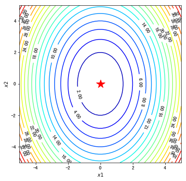
2.2 绘制等高线和梯度场
contour 方法能够绘制等高线,clabel 能够将对应线的高度(函数值)显示出来,这里我们保留两位小数(fmt='%.2f')。
dz_dx1 = elementwise_grad(f1, argnum=0)(x1, x2)
dz_dx2 = elementwise_grad(f1, argnum=1)(x1, x2)
fig, ax = plt.subplots(figsize=(6, 6))

contour = ax.contour(x1, x2, z,levels=20,cmap=plt.cm.jet)
ax.clabel(contour,fontsize=10,colors='k',fmt='%.2f')
ax.plot(*minima, 'r*', markersize=18)

ax.set_xlabel('$x1$')
ax.set_ylabel('$x2$')

ax.set_xlim((-5, 5))
ax.set_ylim((-5, 5))

plt.show()
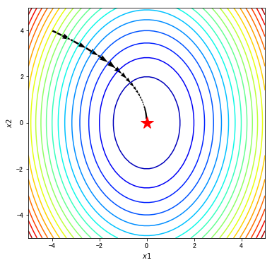
2.3 梯度下降法求解路径二维动画可视化
借助 quiver 函数,我们可以将梯度下降法得到的优化路径使用箭头连接进行可视化。
fig, ax = plt.subplots(figsize=(6, 6))

ax.contour(x1, x2, z, levels=20,cmap=plt.cm.jet)#等高线
#绘制轨迹箭头
ax.quiver(path_list_gd[:-1,0], path_list_gd[:-1,1], path_list_gd[1:,0]-path_list_gd[:-1,0], path_list_gd[1:,1]-path_list_gd[:-1,1], scale_units='xy', angles='xy', scale=1, color='k')
#标注最优值点
ax.plot(*minima, 'r*', markersize=18)

ax.set_xlabel('$x1$')
ax.set_ylabel('$x2$')

ax.set_xlim((-5, 5))
ax.set_ylim((-5, 5))
plt.show()
使用动画将每一步的路径展示出来,我们使用 animation.FuncAnimation 类来完成动画模拟,然后使用 .to_jshtml 方法将动画显示出来。
path = path_list_gd #梯度下降法的优化路径
fig, ax = plt.subplots(figsize=(6, 6))
line, = ax.plot([], [], 'b', label='Gradient Descent', lw=2) #保存路径
point, = ax.plot([], [], 'bo') #保存路径最后的点

def init_draw():
    ax.contour(x1, x2, z, levels=20, cmap=plt.cm.jet)
    ax.plot(*minima, 'r*', markersize=18) #将最小值点绘制成红色五角星
    ax.set_xlabel('$x$')
    ax.set_ylabel('$y$')
    ax.set_xlim((-5, 5))
    ax.set_ylim((-5, 5))
    return line, point

def update_draw(i):
    line.set_data(path[:i,0],path[:i,1])
    point.set_data(path[i-1:i,0],path[i-1:i,1])
    plt.close()
    return line, point

anim = animation.FuncAnimation(fig, update_draw, init_func=init_draw,frames=path.shape[0], interval=60, repeat_delay=5, blit=True)
HTML(anim.to_jshtml())
3 不同优化方法对比
使用 `scipy.optimize`[1] 模块求解最优化问题。由于我们需要对优化路径进行可视化,因此 minimize 函数需要制定一个回调函数参数 callback。
x0 = np.array([-4, 4])
def make_minimize_cb(path=[]):

    def minimize_cb(xk):
        path.append(np.copy(xk))

    return minimize_cb
3.1 选取不同的优化方法求解
在这里我们选取 scipy.optimize 模块实现的一些常见的优化方法。
methods = [ "CG", "BFGS","Newton-CG","L-BFGS-B"]
import warnings
warnings.filterwarnings('ignore') #该行代码的作用是隐藏警告信息
x0 = [-4.0,4.0]
paths = []
zpaths = []
for method in methods:
    path = [x0]
    res = minimize(fun=f1_grad, x0=x0,jac=True,method = method,callback=make_minimize_cb(path), bounds=[(-5, 5), (-5, 5)], tol=1e-20)
    paths.append(np.array(path))
增加我们自己实现的梯度下降法的结果。
methods.append("GD")
paths.append(path_list_gd)
zpaths = [f1(path[:,0],path[:,1]) for path in paths]
3.2 实现动画演示封装类
封装一个 TrajectoryAnimation 类 ,将不同算法得到的优化路径进行动画演示。本代码来自 louistiao.me[2]。
class TrajectoryAnimation(animation.FuncAnimation):

    def __init__(self, paths, labels=[], fig=None, ax=None, frames=None,
                 interval=60, repeat_delay=5, blit=True, **kwargs):
        #如果传入的fig和ax参数为空,则新建一个fig对象和ax对象
        if fig is None:
            if ax is None:
                fig, ax = plt.subplots()
            else:
                fig = ax.get_figure()
        else:
            if ax is None:
                ax = fig.gca()
        self.fig = fig
        self.ax = ax
        self.paths = paths
        #动画的帧数等于最长的路径长度
        if frames is None:
            frames = max(path.shape[0] for path in paths) #获取最长的路径长度
        self.lines = [ax.plot([], [], label=label, lw=2)[0]
                      for _, label in zip_longest(paths, labels)]
        self.points = [ax.plot([], [], 'o', color=line.get_color())[0]
                       for line in self.lines]
        super(TrajectoryAnimation, self).__init__(fig, self.animate, init_func=self.init_anim,
                                                  frames=frames, interval=interval, blit=blit,
                                                  repeat_delay=repeat_delay, **kwargs)
    def init_anim(self):
        for line, point in zip(self.lines, self.points):
            line.set_data([], [])
            point.set_data([], [])
        return self.lines + self.points

    def animate(self, i):
        for line, point, path in zip(self.lines, self.points, self.paths):
            line.set_data(path[:i,0],path[:i,1])
            point.set_data(path[i-1:i,0],path[i-1:i,1])
            plt.close()
        return self.lines + self.points
3.3 求解路径的对比
fig, ax = plt.subplots(figsize=(8, 8))

ax.contour(x1, x2, z, cmap=plt.cm.jet)
ax.plot(*minima, 'r*', markersize=10)

ax.set_xlabel('$x1$')
ax.set_ylabel('$x2$')

ax.set_xlim((-5, 5))
ax.set_ylim((-5, 5))

anim = TrajectoryAnimation(paths, labels=methods, ax=ax)

ax.legend(loc='upper left')
HTML(anim.to_jshtml())
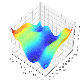
3.4 复杂函数优化的对比
我们再来看一个有多个局部最小值和鞍点的函数。
f2 = lambda x1, x2 :((4 - 2.1*x1**2 + x1**4 / 3.) * x1**2 + x1 * x2  + (-4 + 4*x2**2) * x2 **2)
f2_grad = value_and_grad(lambda args: f2(*args))

x1,x2 = np.meshgrid(np.linspace(-2.0,2.0,50), np.linspace(-1.0,1.0,50))
z = f2(x1,x2 )

%matplotlib inline
fig = plt.figure(figsize=(6, 6))
ax = plt.axes(projection='3d', elev=50, azim=-50)

ax.plot_surface(x1,x2, z, alpha=.8, cmap=plt.cm.jet)

ax.set_xlabel('$x1$')
ax.set_ylabel('$x2$')
ax.set_zlabel('$f$')

ax.set_xlim((-2.0, 2.0))
ax.set_ylim((-1.0, 1.0))

plt.show()
使用 Scipy 中实现的不同的优化方法以及我们在本案例实现的梯度下降法进行求解。
x02 = [-1.0,-0.5]  #初始点,尝试不同初始点,[-1.0,-0.5] ,[1.5,0.75],[-0.8,0.25]
_, path_list_gd2 = gradient_descent(f2,f2_grad,x02,0.1,30) #使用梯度下降法求解

paths = []
zpaths = []
methods = [ "CG", "BFGS","Newton-CG","L-BFGS-B"]
for method in methods:
    path = [x02]
    res = minimize(fun=f2_grad, x0=x02,jac=True,method = method,callback=make_minimize_cb(path), bounds=[(-2.0, 2.0), (-1.0, 1.0)], tol=1e-20)
    paths.append(np.array(path))

methods.append("GD")
paths.append(path_list_gd2)
zpaths = [f2(path[:,0],path[:,1]) for path in paths]
将不同方法的求解路径以动画形式显示出来。
%matplotlib inline
fig, ax = plt.subplots(figsize=(8, 8))

contour = ax.contour(x1, x2, z, levels=50, cmap=plt.cm.jet)
ax.clabel(contour,fontsize=10,colors='k',fmt='%.2f')
ax.set_xlabel('$x1$')
ax.set_ylabel('$x2$')

ax.set_xlim((-2.0, 2.0))
ax.set_ylim((-1.0, 1.0))

anim = TrajectoryAnimation(paths, labels=methods, ax=ax)
ax.legend(loc='upper left')
HTML(anim.to_jshtml())
4 使用不同的优化算法求解手写数字分类问题
4.1 手写数字数据加载和预处理
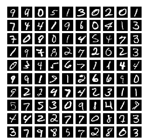
MNIST 手写数字数据集是在图像处理和深度学习领域一个著名的图像数据集。该数据集包含一份 60000 个图像样本的训练集和包含 10000 个图像样本的测试集。每一个样本是 的图像,每个图像有一个标签,标签取值为 0-9 。MNIST 数据集下载地址为 http://yann.lecun.com/exdb/mnist/[3]。
import numpy as np
f = np.load("input/mnist.npz")
X_train, y_train, X_test, y_test = f['x_train'], f['y_train'],f['x_test'], f['y_test']
f.close()
x_train = X_train.reshape((-1, 28*28)) / 255.0
x_test = X_test.reshape((-1, 28*28)) / 255.0
随机打印一些手写数字,查看数据集。
rndperm = np.random.permutation(len(x_train))
%matplotlib inline
import matplotlib.pyplot as plt
plt.gray()
fig = plt.figure( figsize=(8,8) )
for i in range(0,100):
    ax = fig.add_subplot(10,10,i+1)
    ax.matshow(x_train[rndperm[i]].reshape((28,28)))
    plt.box(False) #去掉边框
    plt.axis("off")#不显示坐标轴
plt.show()
< Figure size 432x288 with 0 Axes >
 为了便于后续模型训练,对手写数字的标签进行 One-Hot 编码。
import pandas as pd
y_train_onehot = pd.get_dummies(y_train)
y_train_onehot.head()
| 0 | 1 | 2 | 3 | 4 | 5 | 6 | 7 | 8 | 9 | |
|---|---|---|---|---|---|---|---|---|---|---|
| 0 | 0 | 0 | 0 | 0 | 0 | 1 | 0 | 0 | 0 | 0 |
| 1 | 1 | 0 | 0 | 0 | 0 | 0 | 0 | 0 | 0 | 0 |
| 2 | 0 | 0 | 0 | 0 | 1 | 0 | 0 | 0 | 0 | 0 |
| 3 | 0 | 1 | 0 | 0 | 0 | 0 | 0 | 0 | 0 | 0 |
| 4 | 0 | 0 | 0 | 0 | 0 | 0 | 0 | 0 | 0 | 1 |
4.2 使用 TensorFlow 构建手写数字识别神经网络
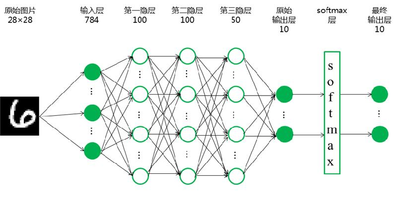
构建一个简单的全连接神经网络,用于手写数字的分类,网络结构如下图所示:
import tensorflow as tf
import tensorflow.keras.layers as layers
现在我们构建上述神经网络,结构为 784->100->100->50->10。
inputs = layers.Input(shape=(28*28,), name='inputs')
hidden1 = layers.Dense(100, activation='relu', name='hidden1')(inputs)
hidden2 = layers.Dense(100, activation='relu', name='hidden2')(hidden1)
hidden3 = layers.Dense(50, activation='relu', name='hidden3')(hidden2)
outputs = layers.Dense(10, activation='softmax', name='outputs')(hidden3)
deep_networks = tf.keras.Model(inputs,outputs)
deep_networks.summary()
_________________________________________________________________
Layer (type)                 Output Shape              Param #
=================================================================
inputs (InputLayer)          (None, 784)               0
_________________________________________________________________
hidden1 (Dense)              (None, 100)               78500
_________________________________________________________________
hidden2 (Dense)              (None, 100)               10100
_________________________________________________________________
hidden3 (Dense)              (None, 50)                5050
_________________________________________________________________
outputs (Dense)              (None, 10)                510
=================================================================
Total params: 94,160
Trainable params: 94,160
Non-trainable params: 0
_________________________________________________________________
4.3 损失函数、优化方法选择与模型训练
deep_networks.compile(optimizer='SGD',loss='categorical_crossentropy',metrics=['accuracy']) #定义误差和优化方法 SGD,RMSprop,Adam,Adagrad,Nadam
%time history = deep_networks.fit(x_train, y_train_onehot, batch_size=500, epochs=10,validation_split=0.5,verbose=1) #模型训练
Train on 30000 samples, validate on 30000 samples Epoch 1/10 30000/30000 [==============================] - 1s 27us/step - loss: 0.0516 - acc: 0.9865 - val_loss: 0.1246 - val_acc: 0.9634 Epoch 2/10 30000/30000 [==============================] - 0s 16us/step - loss: 0.0502 - acc: 0.9869 - val_loss: 0.1243 - val_acc: 0.9634 Epoch 3/10 30000/30000 [==============================] - 0s 16us/step - loss: 0.0496 - acc: 0.9871 - val_loss: 0.1244 - val_acc: 0.9634 Epoch 4/10 30000/30000 [==============================] - 0s 16us/step - loss: 0.0492 - acc: 0.9874 - val_loss: 0.1244 - val_acc: 0.9634 Epoch 5/10 30000/30000 [==============================] - 0s 16us/step - loss: 0.0489 - acc: 0.9875 - val_loss: 0.1247 - val_acc: 0.9633 Epoch 6/10 30000/30000 [==============================] - 0s 16us/step - loss: 0.0485 - acc: 0.9873 - val_loss: 0.1244 - val_acc: 0.9635 Epoch 7/10 30000/30000 [==============================] - 0s 16us/step - loss: 0.0483 - acc: 0.9873 - val_loss: 0.1244 - val_acc: 0.9637 Epoch 8/10 30000/30000 [==============================] - 0s 16us/step - loss: 0.0479 - acc: 0.9878 - val_loss: 0.1242 - val_acc: 0.9636 Epoch 9/10 30000/30000 [==============================] - 0s 16us/step - loss: 0.0477 - acc: 0.9874 - val_loss: 0.1245 - val_acc: 0.9636 Epoch 10/10 30000/30000 [==============================] - 0s 17us/step - loss: 0.0475 - acc: 0.9874 - val_loss: 0.1245 - val_acc: 0.9637 CPU times: user 17.8 s, sys: 2.08 s, total: 19.8 s Wall time: 5.36 s
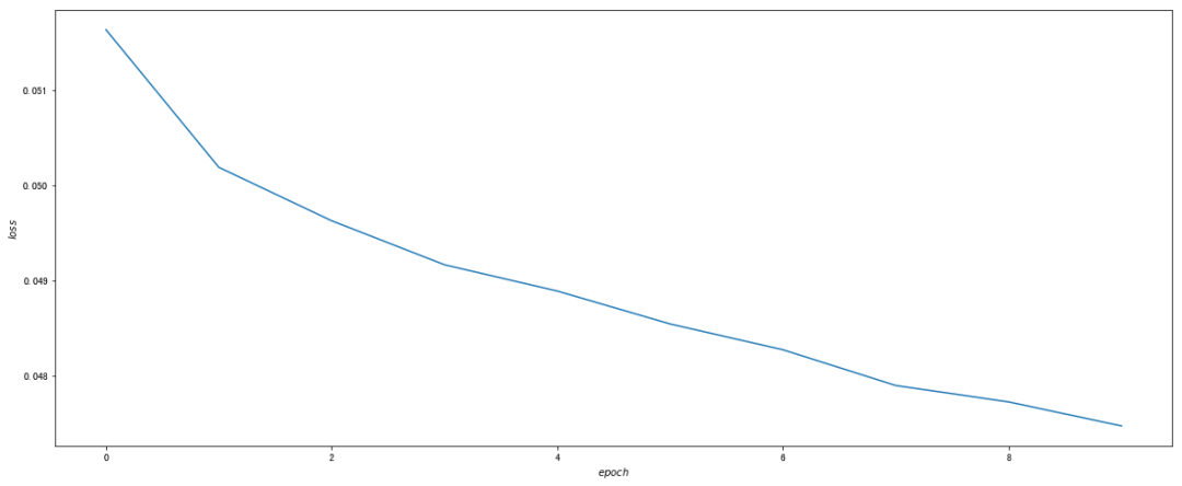
打印误差变化曲线。
fig, ax = plt.subplots(figsize=(20, 8))

ax.plot(history.epoch, history.history["loss"])

ax.set_xlabel('$epoch$')
ax.set_ylabel('$loss$')
Text(0, 0.5, '$loss$')
test_loss, test_acc = deep_networks.evaluate(x_test,  pd.get_dummies(y_test), verbose=2)

print('\nTest accuracy:', test_acc)
Test accuracy: 0.9667
5 总结
本案例我们实现了梯度下降法,借助 Scipy 的 optimize 模块,在两个不同的二维函数上使用梯度下降、共轭梯度下降法和拟牛顿法的优化路径,并使用 Matplotlib 进行了动画展示。然后在手写数字数据集上,我们使用 TensorFlow 构建分类模型,使用不同的优化方法进行模型训练。本案例主要用到的 Python 包列举如下。
| 包或方法 | 版本 | 用途 |
|---|---|---|
| Matplotlib | 3.0.2 | 绘制三维曲面,绘制等高线,制作动画,绘制梯度场(箭头 |
| Scipy | 1.0.0 | scipy.optimize.minimize 求解最优化问题 |
| TensorFlow | 1.12.0 | 构建手写数字神经网络模型 |
| Pandas | 0.23.4 | 数据预处理,One-Hot 编码 |
参考资料
[1]scipy.optimize: http://docs.scipy.org/doc/scipy/reference/optimize.html
louistiao.me: http://louistiao.me/notes/visualizing-and-animating-optimization-algorithms-with-matplotlib/
[3]http://yann.lecun.com/exdb/mnist/: http://yann.lecun.com/exdb/mnist/
机器学习十讲往期直播案例
直播案例 |使用PageRank对全球机场进行排序
直播案例 |使用KNN对新闻主题进行自动分类
直播案例 |使用回归模型预测鲍鱼年龄
直播案例 |使用感知机、逻辑回归、支持向量机进行中文新闻主题分类
直播案例 |决策树、随机森林和 AdaBoost 的 Python 实现
直播案例 | K-Means 的 Python 实现及在图像分割和新闻聚类中的应用
直播案例 |Python 降维实践及在特征脸、图像重构和文本数据中的应用
机器学习十讲直播课件

/机器会学习吗?
05/14---机器学习介绍

/回归初心,方得始终
05/21---回归

/分门别类,各得其所
05/28---分类

/三个臭皮匠,顶个诸葛亮
06/04---模型提升

/物以类聚,人以群分
06/11---聚类

/取其精华,去其糟粕
06/18---降维


 741
741


 被折叠的 条评论
为什么被折叠?
被折叠的 条评论
为什么被折叠?
 到【灌水乐园】发言


