matlab车道线检测_项目实践 | 酷炫项目免费拿！车辆距离与车道线检测项目实践...

点击最上方蓝色【AI算法修炼营】关注公众号

回复【车辆检测】即可获得完整的项目代码以及文档说明。

1、项目流程的简介

   项目的主题框架使用为Keras+OpenCV的形式实现，而模型的选择为基于DarkNet19的YOLO V2模型，权重为基于COCO2014训练的数据集，而车道线的检测是基于OpenCV的传统方法实现的。

2、项目主题部分

2.1、YOLO V2模型

    YoloV2的结构是比较简单的，这里要注意的地方有两个：

    1.输出的是batchsize x (5+20)*5 x W x H的feature map；

      2.这里为了提取细节，加了一个 Fine-Grained connection layer，将前面的细节信息汇聚到了后面的层当中。

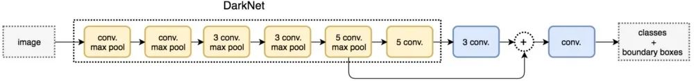
YOLOv2结构示意图

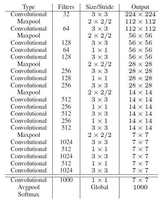
2.1.1、DarkNet19模型

    YOLOv2采用了一个新的基础模型(特征提取器)，称为Darknet-19，包括19个卷积层和5个maxpooling层；Darknet-19与VGG16模型设计原则是一致的，主要采用3*3卷积，采用 2*2的maxpooling层之后，特征图维度降低2倍，而同时将特征图的channles增加两倍。

    与NIN(Network in Network)类似，Darknet-19最终采用global avgpooling做预测，并且在3*3卷积之间使用1*1卷积来压缩特征图channles以降低模型计算量和参数。

    Darknet-19每个卷积层后面同样使用了batch norm层以加快收敛速度，降低模型过拟合。在ImageNet分类数据集上，Darknet-19的top-1准确度为72.9%，top-5准确度为91.2%，但是模型参数相对小一些。使用Darknet-19之后，YOLOv2的mAP值没有显著提升，但是计算量却可以减少约33%。

"""Darknet19 Model Defined in Keras."""import functoolsfrom functools import partialfrom keras.layers import Conv2D, MaxPooling2Dfrom keras.layers.advanced_activations import LeakyReLUfrom keras.layers.normalization import BatchNormalizationfrom keras.models import Modelfrom keras.regularizers import l2from ..utils import compose# Partial wrapper for Convolution2D with static default argument._DarknetConv2D = partial(Conv2D, padding='same')@functools.wraps(Conv2D)def DarknetConv2D(*args, **kwargs):    """Wrapper to set Darknet weight regularizer for Convolution2D."""    darknet_conv_kwargs = {'kernel_regularizer': l2(5e-4)}    darknet_conv_kwargs.update(kwargs)    return _DarknetConv2D(*args, **darknet_conv_kwargs)def DarknetConv2D_BN_Leaky(*args, **kwargs):    """Darknet Convolution2D followed by BatchNormalization and LeakyReLU."""    no_bias_kwargs = {'use_bias': False}    no_bias_kwargs.update(kwargs)    return compose(        DarknetConv2D(*args, **no_bias_kwargs),        BatchNormalization(),        LeakyReLU(alpha=0.1))def bottleneck_block(outer_filters, bottleneck_filters):    """Bottleneck block of 3x3, 1x1, 3x3 convolutions."""    return compose(        DarknetConv2D_BN_Leaky(outer_filters, (3, 3)),        DarknetConv2D_BN_Leaky(bottleneck_filters, (1, 1)),        DarknetConv2D_BN_Leaky(outer_filters, (3, 3)))def bottleneck_x2_block(outer_filters, bottleneck_filters):    """Bottleneck block of 3x3, 1x1, 3x3, 1x1, 3x3 convolutions."""    return compose(        bottleneck_block(outer_filters, bottleneck_filters),        DarknetConv2D_BN_Leaky(bottleneck_filters, (1, 1)),        DarknetConv2D_BN_Leaky(outer_filters, (3, 3)))def darknet_body():    """Generate first 18 conv layers of Darknet-19."""    return compose(        DarknetConv2D_BN_Leaky(32, (3, 3)),        MaxPooling2D(),        DarknetConv2D_BN_Leaky(64, (3, 3)),        MaxPooling2D(),        bottleneck_block(128, 64),        MaxPooling2D(),        bottleneck_block(256, 128),        MaxPooling2D(),        bottleneck_x2_block(512, 256),        MaxPooling2D(),        bottleneck_x2_block(1024, 512))def darknet19(inputs):    """Generate Darknet-19 model for Imagenet classification."""    body = darknet_body()(inputs)    logits = DarknetConv2D(1000, (1, 1), activation='softmax')(body)    return Model(inputs, logits)

2.1.2、Fine-Grained Features

    YOLOv2的输入图片大小为416*416，经过5次maxpooling之后得到13*13大小的特征图，并以此特征图采用卷积做预测。13*13大小的特征图对检测大物体是足够了，但是对于小物体还需要更精细的特征图(Fine-Grained Features)。因此SSD使用了多尺度的特征图来分别检测不同大小的物体，前面更精细的特征图可以用来预测小物体。

    YOLOv2提出了一种passthrough层来利用更精细的特征图。YOLOv2所利用的Fine-Grained Features是26*26大小的特征图(最后一个maxpooling层的输入)，对于Darknet-19模型来说就是大小为 26*26*512的特征图。passthrough层与ResNet网络的shortcut类似，以前面更高分辨率的特征图为输入，然后将其连接到后面的低分辨率特征图上。前面的特征图维度是后面的特征图的2倍，passthrough层抽取前面层的每个2*2的局部区域，然后将其转化为channel维度，对于26*26*512的特征图，经passthrough层处理之后就变成了13*13*2048的新特征图(特征图大小降低4倍，而channles增加4倍，图6为一个实例)，这样就可以与后面的13*13*1024特征图连接在一起形成13*13*3072大小的特征图，然后在此特征图基础上卷积做预测。

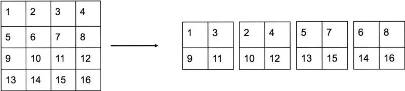
passthrough层实例

    另外，作者在后期的实现中借鉴了ResNet网络，不是直接对高分辨特征图处理，而是增加了一个中间卷积层，先采用64个 1*1卷积核进行卷积，然后再进行passthrough处理，这样26*26*512的特征图得到13*13*256的特征图。

    这算是实现上的一个小细节。使用Fine-Grained Features之后YOLOv2的性能有1%的提升。

2.1.3、Dimension Clusters

    在Faster R-CNN和SSD中，先验框的维度(长和宽)都是手动设定的，带有一定的主观性。如果选取的先验框维度比较合适，那么模型更容易学习，从而做出更好的预测。因此，YOLOv2采用k-means聚类方法对训练集中的边界框做了聚类分析。

    因为设置先验框的主要目的是为了使得预测框与ground truth的IOU更好，所以聚类分析时选用box与聚类中心box之间的IOU值作为距离指标。

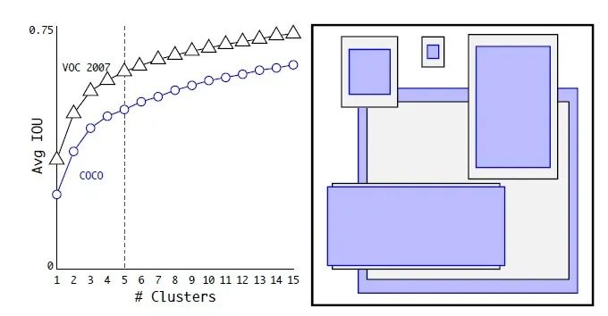
数据集VOC和COCO上的边界框聚类分析结果

2.1.4、YOLOv2的训练

    YOLOv2的训练主要包括三个阶段。第一阶段就是先在coco分类数据集上预训练Darknet-19，此时模型输入为224*224，共训练160个epochs。然后第二阶段将网络的输入调整为448*448，继续在ImageNet数据集上finetune分类模型，训练10个epochs，此时分类模型的top-1准确度为76.5%，而top-5准确度为93.3%。第三个阶段就是修改Darknet-19分类模型为检测模型，并在检测数据集上继续finetune网络。

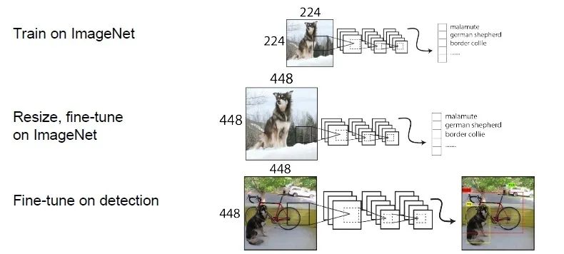
YOLOv2训练的三个阶段

loss计算公式：

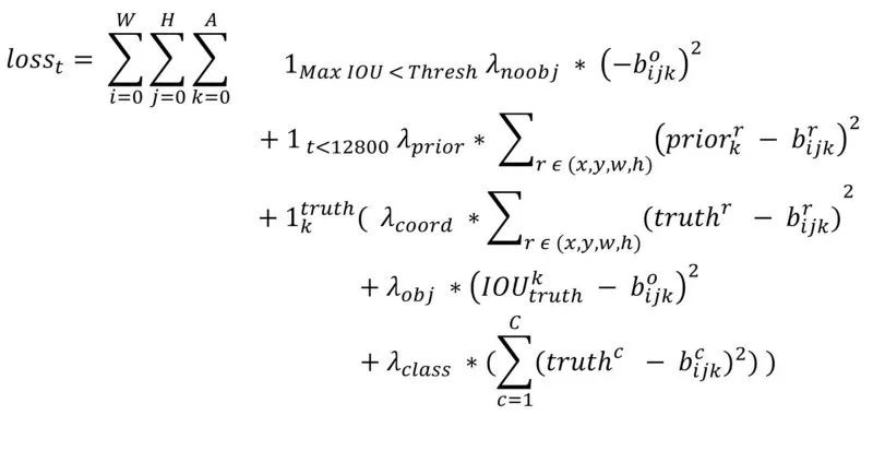
def yolo_loss(args,              anchors,              num_classes,              rescore_confidence=False,              print_loss=False):    """YOLO localization loss function.    Parameters    ----------    yolo_output : tensor        Final convolutional layer features.    true_boxes : tensor        Ground truth boxes tensor with shape [batch, num_true_boxes, 5]        containing box x_center, y_center, width, height, and class.    detectors_mask : array        0/1 mask for detector positions where there is a matching ground truth.    matching_true_boxes : array        Corresponding ground truth boxes for positive detector positions.        Already adjusted for conv height and width.    anchors : tensor        Anchor boxes for model.    num_classes : int        Number of object classes.    rescore_confidence : bool, default=False        If true then set confidence target to IOU of best predicted box with        the closest matching ground truth box.    print_loss : bool, default=False        If True then use a tf.Print() to print the loss components.    Returns    -------    mean_loss : float        mean localization loss across minibatch    """    (yolo_output, true_boxes, detectors_mask, matching_true_boxes) = args    num_anchors = len(anchors)    object_scale = 5    no_object_scale = 1    class_scale = 1    coordinates_scale = 1    pred_xy, pred_wh, pred_confidence, pred_class_prob = yolo_head(        yolo_output, anchors, num_classes)    # Unadjusted box predictions for loss.    # TODO: Remove extra computation shared with yolo_head.    yolo_output_shape = K.shape(yolo_output)    feats = K.reshape(yolo_output, [        -1, yolo_output_shape[1], yolo_output_shape[2], num_anchors,        num_classes + 5    ])    pred_boxes = K.concatenate(        (K.sigmoid(feats[..., 0:2]), feats[..., 2:4]), axis=-1)    # TODO: Adjust predictions by image width/height for non-square images?    # IOUs may be off due to different aspect ratio.    # Expand pred x,y,w,h to allow comparison with ground truth.    # batch, conv_height, conv_width, num_anchors, num_true_boxes, box_params    pred_xy = K.expand_dims(pred_xy, 4)    pred_wh = K.expand_dims(pred_wh, 4)    pred_wh_half = pred_wh / 2.    pred_mins = pred_xy - pred_wh_half    pred_maxes = pred_xy + pred_wh_half    true_boxes_shape = K.shape(true_boxes)    # batch, conv_height, conv_width, num_anchors, num_true_boxes, box_params    true_boxes = K.reshape(true_boxes, [        true_boxes_shape[0], 1, 1, 1, true_boxes_shape[1], true_boxes_shape[2]    ])    true_xy = true_boxes[..., 0:2]    true_wh = true_boxes[..., 2:4]    # Find IOU of each predicted box with each ground truth box.    true_wh_half = true_wh / 2.    true_mins = true_xy - true_wh_half    true_maxes = true_xy + true_wh_half    intersect_mins = K.maximum(pred_mins, true_mins)    intersect_maxes = K.minimum(pred_maxes, true_maxes)    intersect_wh = K.maximum(intersect_maxes - intersect_mins, 0.)    intersect_areas = intersect_wh[..., 0] * intersect_wh[..., 1]    pred_areas = pred_wh[..., 0] * pred_wh[..., 1]    true_areas = true_wh[..., 0] * true_wh[..., 1]    union_areas = pred_areas + true_areas - intersect_areas    iou_scores = intersect_areas / union_areas    # Best IOUs for each location.    best_ious = K.max(iou_scores, axis=4)  # Best IOU scores.    best_ious = K.expand_dims(best_ious)    # A detector has found an object if IOU > thresh for some true box.    object_detections = K.cast(best_ious > 0.6, K.dtype(best_ious))    # TODO: Darknet region training includes extra coordinate loss for early    # training steps to encourage predictions to match anchor priors.    # Determine confidence weights from object and no_object weights.    # NOTE: YOLO does not use binary cross-entropy here.    no_object_weights = (no_object_scale * (1 - object_detections) *                         (1 - detectors_mask))    no_objects_loss = no_object_weights * K.square(-pred_confidence)    if rescore_confidence:        objects_loss = (object_scale * detectors_mask *                        K.square(best_ious - pred_confidence))    else:        objects_loss = (object_scale * detectors_mask *                        K.square(1 - pred_confidence))    confidence_loss = objects_loss + no_objects_loss    # Classification loss for matching detections.    # NOTE: YOLO does not use categorical cross-entropy loss here.    matching_classes = K.cast(matching_true_boxes[..., 4], 'int32')    matching_classes = K.one_hot(matching_classes, num_classes)    classification_loss = (class_scale * detectors_mask *                           K.square(matching_classes - pred_class_prob))    # Coordinate loss for matching detection boxes.    matching_boxes = matching_true_boxes[..., 0:4]    coordinates_loss = (coordinates_scale * detectors_mask *                        K.square(matching_boxes - pred_boxes))    confidence_loss_sum = K.sum(confidence_loss)    classification_loss_sum = K.sum(classification_loss)    coordinates_loss_sum = K.sum(coordinates_loss)    total_loss = 0.5 * (        confidence_loss_sum + classification_loss_sum + coordinates_loss_sum)    if print_loss:        total_loss = tf.Print(            total_loss, [                total_loss, confidence_loss_sum, classification_loss_sum,                coordinates_loss_sum            ],            message='yolo_loss, conf_loss, class_loss, box_coord_loss:')    return total_loss

2.2、车距的计算

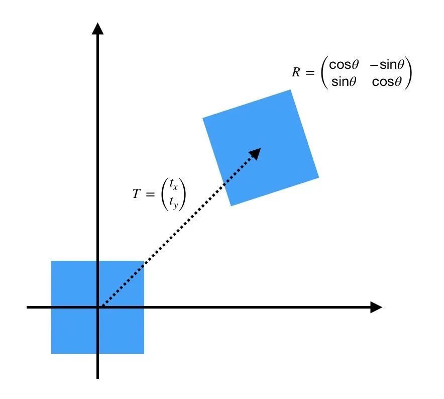
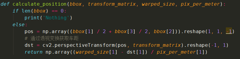
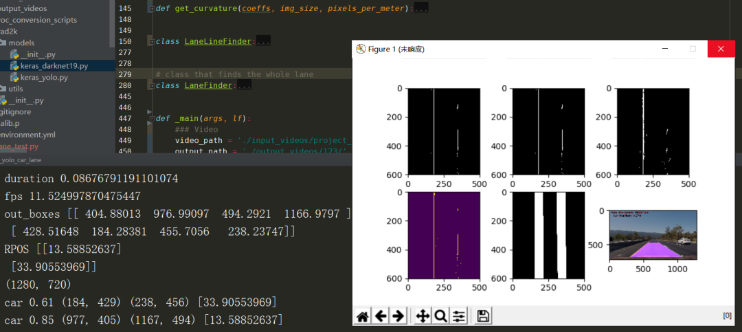
    通过YOLO进行检测车量，然后返回的车辆检测框的坐标与当前坐标进行透视变换获取大约的距离作为车辆之间的距离。

    所使用的函数API接口为：

cv2.perspectiveTransform(src, m[, dst]) → dst

参数解释

    •src：输入的2通道或者3通道的图片

    •m：变换矩阵

    返回距离

代码：

2.3、车道线的分割

车道线检测的流程：

实现步骤：

1. 图片校正(对于相机畸变较大的需要先计算相机的畸变矩阵和失真系数，对图片进行校正)；

2. 截取感兴趣区域，仅对包含车道线信息的图像区域进行处理；

3. 使用透视变换，将感兴趣区域图片转换成鸟瞰图；

4. 针对不同颜色的车道线，不同光照条件下的车道线，不同清晰度的车道线，根据不同的颜色空间使用不同的梯度阈值，颜色阈值进行不同的处理。并将每一种处理方式进行融合，得到车道线的二进制图；

5. 提取二进制图中属于车道线的像素；

6. 对二进制图片的像素进行直方图统计，统计左右两侧的峰值点作为左右车道线的起始点坐标进行曲线拟合；

7. 使用二次多项式分别拟合左右车道线的像素点(对于噪声较大的像素点，可以进行滤波处理，或者使用随机采样一致性算法进行曲线拟合)；

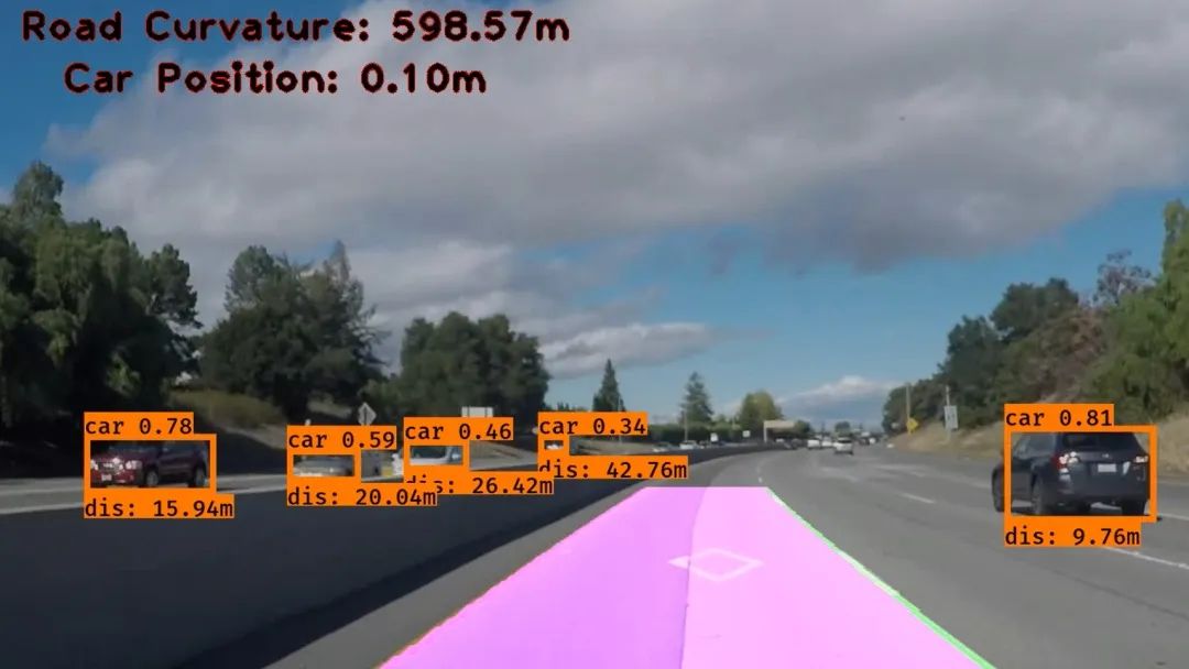
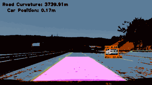
8. 计算车道曲率及车辆相对车道中央的偏离位置；

9. 效果显示(可行域显示，曲率和位置显示)。

# class that finds the whole laneclass LaneFinder:    def __init__(self, img_size, warped_size, cam_matrix, dist_coeffs, transform_matrix, pixels_per_meter,                 warning_icon):        self.found = False        self.cam_matrix = cam_matrix        self.dist_coeffs = dist_coeffs        self.img_size = img_size        self.warped_size = warped_size        self.mask = np.zeros((warped_size[1], warped_size[0], 3), dtype=np.uint8)        self.roi_mask = np.ones((warped_size[1], warped_size[0], 3), dtype=np.uint8)        self.total_mask = np.zeros_like(self.roi_mask)        self.warped_mask = np.zeros((self.warped_size[1], self.warped_size[0]), dtype=np.uint8)        self.M = transform_matrix        self.count = 0        self.left_line = LaneLineFinder(warped_size, pixels_per_meter, -1.8288)  # 6 feet in meters        self.right_line = LaneLineFinder(warped_size, pixels_per_meter, 1.8288)        if (warning_icon is not None):            self.warning_icon = np.array(mpimg.imread(warning_icon) * 255, dtype=np.uint8)        else:            self.warning_icon = None    def undistort(self, img):        return cv2.undistort(img, self.cam_matrix, self.dist_coeffs)    def warp(self, img):        return cv2.warpPerspective(img, self.M, self.warped_size, flags=cv2.WARP_FILL_OUTLIERS + cv2.INTER_CUBIC)    def unwarp(self, img):        return cv2.warpPerspective(img, self.M, self.img_size, flags=cv2.WARP_FILL_OUTLIERS +                                                                     cv2.INTER_CUBIC + cv2.WARP_INVERSE_MAP)    def equalize_lines(self, alpha=0.9):        mean = 0.5 * (self.left_line.coeff_history[:, 0] + self.right_line.coeff_history[:, 0])        self.left_line.coeff_history[:, 0] = alpha * self.left_line.coeff_history[:, 0] + \                                             (1 - alpha) * (mean - np.array([0, 0, 1.8288], dtype=np.uint8))        self.right_line.coeff_history[:, 0] = alpha * self.right_line.coeff_history[:, 0] + \                                              (1 - alpha) * (mean + np.array([0, 0, 1.8288], dtype=np.uint8))    def find_lane(self, img, distorted=True, reset=False):        # undistort, warp, change space, filter        if distorted:            img = self.undistort(img)        if reset:            self.left_line.reset_lane_line()            self.right_line.reset_lane_line()        img = self.warp(img)        img_hls = cv2.cvtColor(img, cv2.COLOR_RGB2HLS)        img_hls = cv2.medianBlur(img_hls, 5)        img_lab = cv2.cvtColor(img, cv2.COLOR_RGB2LAB)        img_lab = cv2.medianBlur(img_lab, 5)        big_kernel = cv2.getStructuringElement(cv2.MORPH_ELLIPSE, (31, 31))        small_kernel = cv2.getStructuringElement(cv2.MORPH_RECT, (7, 7))        greenery = (img_lab[:, :, 2].astype(np.uint8) > 130) & cv2.inRange(img_hls, (0, 0, 50), (138, 43, 226))        road_mask = np.logical_not(greenery).astype(np.uint8) & (img_hls[:, :, 1] < 250)        road_mask = cv2.morphologyEx(road_mask, cv2.MORPH_OPEN, small_kernel)        road_mask = cv2.dilate(road_mask, big_kernel)        img2, contours, hierarchy = cv2.findContours(road_mask, cv2.RETR_LIST, cv2.CHAIN_APPROX_NONE)        biggest_area = 0        for contour in contours:            area = cv2.contourArea(contour)            if area > biggest_area:                biggest_area = area                biggest_contour = contour        road_mask = np.zeros_like(road_mask)        cv2.fillPoly(road_mask, [biggest_contour], 1)        self.roi_mask[:, :, 0] = (self.left_line.line_mask | self.right_line.line_mask) & road_mask        self.roi_mask[:, :, 1] = self.roi_mask[:, :, 0]        self.roi_mask[:, :, 2] = self.roi_mask[:, :, 0]        kernel = cv2.getStructuringElement(cv2.MORPH_ELLIPSE, (7, 3))        black = cv2.morphologyEx(img_lab[:, :, 0], cv2.MORPH_TOPHAT, kernel)        lanes = cv2.morphologyEx(img_hls[:, :, 1], cv2.MORPH_TOPHAT, kernel)        kernel = cv2.getStructuringElement(cv2.MORPH_RECT, (13, 13))        lanes_yellow = cv2.morphologyEx(img_lab[:, :, 2], cv2.MORPH_TOPHAT, kernel)        self.mask[:, :, 0] = cv2.adaptiveThreshold(black, 1, cv2.ADAPTIVE_THRESH_MEAN_C, cv2.THRESH_BINARY, 13, -6)        self.mask[:, :, 1] = cv2.adaptiveThreshold(lanes, 1, cv2.ADAPTIVE_THRESH_MEAN_C, cv2.THRESH_BINARY, 13, -4)        self.mask[:, :, 2] = cv2.adaptiveThreshold(lanes_yellow, 1, cv2.ADAPTIVE_THRESH_MEAN_C, cv2.THRESH_BINARY,13, -1.5)        self.mask *= self.roi_mask        small_kernel = cv2.getStructuringElement(cv2.MORPH_ELLIPSE, (3, 3))        self.total_mask = np.any(self.mask, axis=2).astype(np.uint8)        self.total_mask = cv2.morphologyEx(self.total_mask.astype(np.uint8), cv2.MORPH_ERODE, small_kernel)        left_mask = np.copy(self.total_mask)        right_mask = np.copy(self.total_mask)        if self.right_line.found:            left_mask = left_mask & np.logical_not(self.right_line.line_mask) & self.right_line.other_line_mask        if self.left_line.found:            right_mask = right_mask & np.logical_not(self.left_line.line_mask) & self.left_line.other_line_mask        self.left_line.find_lane_line(left_mask, reset)        self.right_line.find_lane_line(right_mask, reset)        self.found = self.left_line.found and self.right_line.found        if self.found:            self.equalize_lines(0.875)    def draw_lane_weighted(self, img, thickness=5, alpha=0.8, beta=1, gamma=0):        left_line = self.left_line.get_line_points()        right_line = self.right_line.get_line_points()        both_lines = np.concatenate((left_line, np.flipud(right_line)), axis=0)        lanes = np.zeros((self.warped_size[1], self.warped_size[0], 3), dtype=np.uint8)        if self.found:            cv2.fillPoly(lanes, [both_lines.astype(np.int32)], (138, 43, 226))            cv2.polylines(lanes, [left_line.astype(np.int32)], False, (255, 0, 255), thickness=thickness)            cv2.polylines(lanes, [right_line.astype(np.int32)], False, (34, 139, 34), thickness=thickness)            cv2.fillPoly(lanes, [both_lines.astype(np.int32)], (138, 43, 226))            mid_coef = 0.5 * (self.left_line.poly_coeffs + self.right_line.poly_coeffs)            curve = get_curvature(mid_coef, img_size=self.warped_size, pixels_per_meter=self.left_line.pixels_per_meter)            shift = get_center_shift(mid_coef, img_size=self.warped_size,                                     pixels_per_meter=self.left_line.pixels_per_meter)            cv2.putText(img, "Road Curvature: {:6.2f}m".format(curve), (20, 50), cv2.FONT_HERSHEY_PLAIN, fontScale=2.5,                        thickness=5, color=(255, 0, 0))            cv2.putText(img, "Road Curvature: {:6.2f}m".format(curve), (20, 50), cv2.FONT_HERSHEY_PLAIN, fontScale=2.5,                        thickness=3, color=(0, 0, 0))            cv2.putText(img, "Car Position: {:4.2f}m".format(shift), (60, 100), cv2.FONT_HERSHEY_PLAIN, fontScale=2.5,                        thickness=5, color=(255, 0, 0))            cv2.putText(img, "Car Position: {:4.2f}m".format(shift), (60, 100), cv2.FONT_HERSHEY_PLAIN, fontScale=2.5,                        thickness=3, color=(0, 0, 0))        else:            warning_shape = self.warning_icon.shape            corner = (10, (img.shape[1] - warning_shape[1]) // 2)            patch = img[corner[0]:corner[0] + warning_shape[0], corner[1]:corner[1] + warning_shape[1]]            patch[self.warning_icon[:, :, 3] > 0] = self.warning_icon[self.warning_icon[:, :, 3] > 0, 0:3]            img[corner[0]:corner[0] + warning_shape[0], corner[1]:corner[1] + warning_shape[1]] = patch            cv2.putText(img, "Lane lost!", (50, 170), cv2.FONT_HERSHEY_PLAIN, fontScale=2.5,                        thickness=5, color=(255, 0, 0))            cv2.putText(img, "Lane lost!", (50, 170), cv2.FONT_HERSHEY_PLAIN, fontScale=2.5,                        thickness=3, color=(0, 0, 0))        lanes_unwarped = self.unwarp(lanes)        return cv2.addWeighted(img, alpha, lanes_unwarped, beta, gamma)    def process_image(self, img, reset=False, show_period=10, blocking=False):        self.find_lane(img, distorted=True, reset=reset)        lane_img = self.draw_lane_weighted(img)        self.count += 1        if show_period > 0 and (self.count % show_period == 1 or show_period == 1):            start = 231            plt.clf()            for i in range(3):                plt.subplot(start + i)                plt.imshow(lf.mask[:, :, i] * 255, cmap='gray')                plt.subplot(234)            plt.imshow((lf.left_line.line + lf.right_line.line) * 255)            ll = cv2.merge((lf.left_line.line, lf.left_line.line * 0, lf.right_line.line))            lm = cv2.merge((lf.left_line.line_mask, lf.left_line.line * 0, lf.right_line.line_mask))            plt.subplot(235)            plt.imshow(lf.roi_mask * 255, cmap='gray')            plt.subplot(236)            plt.imshow(lane_img)            if blocking:                plt.show()            else:                plt.draw()                plt.pause(0.000001)        return lane_img

2.4、测试过程和结果

Gif文件由于压缩问题看上不不是很好，后续会对每一部分的内容进行更加细致的实践和讲解。

参考：

https://zhuanlan.zhihu.com/p/35325884

https://www.cnblogs.com/YiXiaoZhou/p/7429481.html

https://github.com/yhcc/yolo2

https://github.com/allanzelener/yad2k

https://zhuanlan.zhihu.com/p/74597564

https://zhuanlan.zhihu.com/p/46295711

https://blog.csdn.net/weixin_38746685/article/details/81613065?depth_1-

https://github.com/yang1688899/CarND-Advanced-Lane-Lines

目标检测系列

秘籍一：模型加速之轻量化网络

秘籍二：非极大值抑制及回归损失优化

秘籍三：多尺度检测

秘籍四：数据增强

秘籍五：解决样本不均衡问题

秘籍六：Anchor-Free

视觉注意力机制系列

Non-local模块与Self-attention之间的关系与区别？

视觉注意力机制用于分类网络：SENet、CBAM、SKNet

Non-local模块与SENet、CBAM的融合：GCNet、DANet

Non-local模块如何改进？来看CCNet、ANN

语义分割系列

一篇看完就懂的语义分割综述

最新实例分割综述：从Mask RCNN 到 BlendMask

超强视频语义分割算法！基于语义流快速而准确的场景解析

CVPR2020 | HANet:通过高度驱动的注意力网络改善城市场景语义分割

基础积累系列

卷积神经网络中的感受野怎么算？

图片中的绝对位置信息，CNN能搞定吗？

理解计算机视觉中的损失函数

深度学习相关的面试考点总结

自动驾驶学习笔记系列

 Apollo Udacity自动驾驶课程笔记——高精度地图、厘米级定位

 Apollo Udacity自动驾驶课程笔记——感知、预测

 Apollo Udacity自动驾驶课程笔记——规划、控制

自动驾驶系统中Lidar和Camera怎么融合？

竞赛与工程项目分享系列

如何让笨重的深度学习模型在移动设备上跑起来

基于Pytorch的YOLO目标检测项目工程大合集

目标检测应用竞赛：铝型材表面瑕疵检测

基于Mask R-CNN的道路物体检测与分割

SLAM系列

视觉SLAM前端：视觉里程计和回环检测

视觉SLAM后端：后端优化和建图模块

视觉SLAM中特征点法开源算法：PTAM、ORB-SLAM

视觉SLAM中直接法开源算法：LSD-SLAM、DSO

视觉SLAM中特征点法和直接法的结合：SVO

2020年最新的iPad Pro上的激光雷达是什么？来聊聊激光SLAM