基于matlab的离散系统时域分析实验,《信号与系统》 实验一 信号的时域分析及Matlab实现...

实验一 信号的时域分析及Matlab实现

参考文章

题目

题目1代码实现

讲解

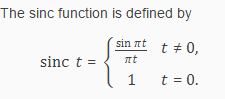
sinc(t)

Sa(t)

时移、翻转、展缩

subs(s,old,new)

ezplot() 绘画符号函数

题目2代码实现

讲解

题目3代码实现

新建函数

单位抽样序列

单位阶跃序列

离散信号的运算

参考文章

信号与系统实验指导

题目

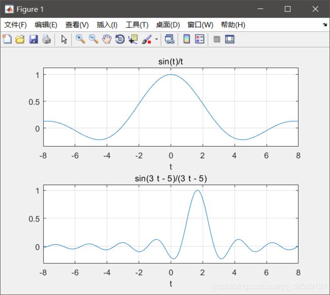
题目1代码实现

syms t;

f=sym('sin(t)/t'); %定义符号函数 f(t)=sin(t)/t

f1=subs(f,t,(-3)*t+5); %对 f 进行移位

subplot(2,1,1);ezplot(f,[-8,8]);grid on;% ezplot 是符号函数绘图命令

subplot(2,1,2);ezplot(f1,[-8,8,-0.3,1.1]);grid on;

运行结果

讲解

sinc(t)

Sa(t)

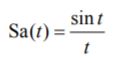
所以sinc (t/pi) = Sa(t)

时移、翻转、展缩

由 f (t)到

f ( − a t + b ) ( a > 0 ) f(-at+b)(a>0)f(−at+b)(a>0)

所用函数

subs(s,old,new)

returns a copy of s replacing all occurrences of old with new, and then evaluating s.

例：已知 f (t) = sin(t) / t ，试通过翻转、移位、展缩由 f (t)的波形得到 f (-2t + 3) 的波形。

syms t;

f=sym('sin(t)/t'); %定义符号函数 f(t)=sin(t)/t

f1=subs(f,t,t+3); %对 f 进行移位

f2=subs(f1,t,2*t); %对 f1 进行展缩

f3=subs(f2,t,-t); %对 f2 进行翻转

可以一步到位

syms t;

f=sym('sin(t)/t'); %定义符号函数 f(t)=sin(t)/t

f3 = subs(f, t, -2t+3);

ezplot() 绘画符号函数

ezplot(fun2,[xmin,xmax,ymin,ymax])

plots fun2(x,y) = 0 over xmin < x < xmax and ymin < y < ymax.

一般搭配使用

subplot(2,1,1);%divides the current figure into an m-by-n grid and creates an axes for a subplot in the position specified by p

ezplot(f,[-8,8,-0.3,1.1]);

grid on;%画网格与否

题目2代码实现

t=(-10:0.01:5);

f1= sin(2*pi*t)+exp(-3*t);

f2= sin(3*pi*t)-exp(-5*t);

f3= sin(2*pi*t).*exp(-3*t);

subplot(2,2,1);plot(t,f1);grid on;

subplot(2,2,2);plot(t,f2);grid on;

subplot(2,2,3);plot(t,f3);grid on;

讲解

f3= sin(2pit).exp(-3t);

如果你使用f3= sin(2pit)exp(-3t);而没加 .,建议学习一下matlab中数组乘法与矩阵乘法的区别

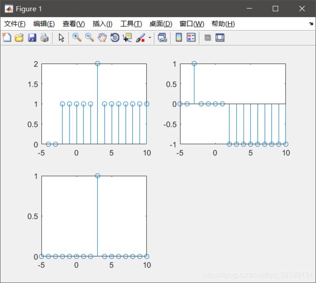
题目3代码实现

[x1,n]=delta(3,-4,10);

[x2,n]=step_seq(-2,-4,10);

subplot(2,2,1);

stem(n,x1+x2);

[x1,n]=delta(-3,-5,10);

[x2,n]=step_seq(2,-5,10);

subplot(2,2,2);

stem(n,x1-x2);

[x1,n]=delta(3,-5,10);

[x2,n]=step_seq(-2,-5,10);

subplot(2,2,3);

stem(n,x1.*x2);

新建函数

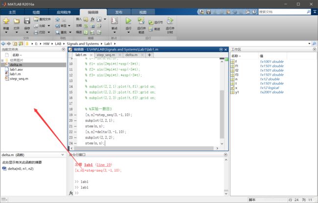
在空白处右键–》新建函数–》函数

修改函数名与文件名一致，最好保存在同一文件夹，到时候在同一个文件夹的其他 .m文件直接引用就ok

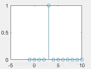
单位抽样序列

δ ( n − n 0 ) = { 1 , n = n 0 0 , n ≠ n 0 \delta(n-n0)=\left\{\begin{array}{lc}1,&n=n0\\0,&n\neq n0\end{array}\right.δ(n−n0)={1,0,​n=n0n​=n0​

先根据上面新建一个函数，然后先定义delta函数，并保存。

function[x,n]=delta(n0,n1 ,n2)

n=[n1:n2];

x=[(n-n0)==0];

然后在主的.m文件

[x,n]=delta(3,-1,10);

stem(n,x);

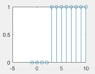
单位阶跃序列

u ( n − n 0 ) = { 1 , n > = n 0 0 , n < n 0 u(n-n0)=\left\{\begin{array}{lc}1,&n>=n0\\0,&nu(n−n0)={1,0,​n>=n0n

先根据上面新建一个函数，然后先定义step_seq函数，并保存。

function[x,n]=step_seq(n0, n1, n2)

n=[n1:n2];

x=[(n-n0)>=0];

然后在主的.m文件

[x,n]=step_seq(3,-1,10);

stem(n,x);

离散信号的运算

n一样，x不一样，在stem里面加

[x1,n]=delta(3,-4,10);

[x2,n]=step_seq(-2,-4,10);

stem(n,x1+x2);

如果是乘法，那么在**“*”前加“.”**