


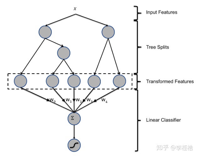
Facebook在2014年的论文Practical Lessons from Predicting Clicks on Ads at Facebook介绍了如何使用GBDT解决LR的特征组合问题,通过GBDT作为树模型具有的路径去构建组合特征,并将组合特征作为LR的输入,从而达到GBDT+LR的融合使用。
下面会介绍如何理解GBDT特征,并用两种方法去提取GBDT特征。用到的数据为Home Credit Default Risk中的application_train.csv。
下面的代码在https://github.com/lizhigu1996/gbdt_var/blob/master/GBDT%E7%89%B9%E5%BE%81%E7%9A%84%E6%8F%90%E5%8F%96%E5%8F%8A%E5%BA%94%E7%94%A8.ipynb中可复现(其他代码是以前写的,没有更新)。
1. GBDT特征的理解
在FaceBook的论文中有个例子,例子中的GBDT是由两棵树组成的,而GBDT特征就是中间虚线那块:
当确定输入样本x后,样本在两棵树中分别经过一条路径,最终分别落到两棵树的叶子节点上。假设有个样本经过的路径如下:
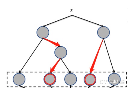
那么该样本的GBDT特征为[0 1 0 1 0],衍生后的GBDT特征就可以直接输入到LR中,这也就是GBDT+LR的融合使用。
2. python实现——模型的apply函数
用实际数据去实现GBDT特征的提取:
application_train = pd.read_csv('data/application_train.csv')
X = application_train[[col for col in application_train.columns if col not in ['SK_ID_CURR', 'TARGET', 'DATE']]]
y = application_train['TARGET']
X_train, X_test, y_train, y_test = train_test_split(X, y, test_size=0.3, random_state=1234)
col_types = X_train.dtypes
char_cols = list(col_types[col_types == 'object'].index)
num_cols = list(col_types[col_types != 'object'].index)
# GradientBoostingClassifier不支持缺失,填充缺失
X_train[char_cols] = X_train[char_cols].fillna('null')
X_train[num_cols] = X_train[num_cols].fillna(-1)
X_test[char_cols] = X_test[char_cols].fillna('null')
X_test[num_cols] = X_test[num_cols].fillna(-1)
# GradientBoostingClassifier不支持类别特征,对类别特征进行ont-hot编码,并使测试集与训练集编码后的特征保持一致
X_train_new = X_train[num_cols].join(pd.get_dummies(X_train[char_cols]))
X_test_new = X_test[num_cols].join(pd.get_dummies(X_test[char_cols]))
for col in set(X_train_new.columns) - set(X_test_new.columns):
X_test_new[col] = 0
X_test_new = X_test_new[X_train_new.columns]
# 训练模型
model = GradientBoostingClassifier(random_state=1234)
model.fit(X_train_new, y_train)
# 获取落到每颗子树的叶子节点结果
train_leaf_feature1 = model.apply(X_train_new)[:, :, 0]
test_leaf_feature1 = model.apply(X_test_new)[:, :, 0]
# 转换成GBDT特征
enc = OneHotEncoder()
enc.fit(train_leaf_feature1)
train_gbdt_feature1 = np.array(enc.transform(train_leaf_feature1).toarray())
test_gbdt_feature1 = np.array(enc.transform(test_leaf_feature1).toarray())下面对训练完模型后如何得到GBDT特征的过程进行分解,首先看model.apply(X_train)[:, :, 0]的结果是什么。
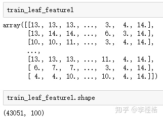
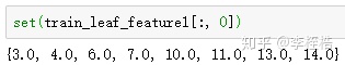
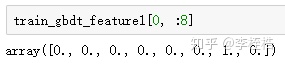
可以看到train_leaf_feature1有100列,由于GradientBoostingClassifier默认生成的子树为100颗,train_leaf_feature1的每一列其实就是对应着样本在每一颗子树落到的叶子节点。
生成第一棵树的可视画图:
import graphviz
dot_data = export_graphviz(model.estimators_[0, 0], out_file=None, feature_names=X_train_new.columns,
                           filled=True, rounded=True, special_characters=True)
graph = graphviz.Source(dot_data)
graph.render('tree1.gv')
得到如下可视化图,节点序号从左到右开始计算,所以叶子节点的序号为[3 4 6 7 10 11 13 14]:
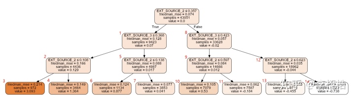
可以看到第一列的取值也只有[3 4 6 7 10 11 13 14]:
可以拿第一个样本验证:
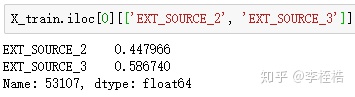
由于第一个样本EXT_SOURCE_2 > 0.357,EXT_SOURCE_3 > 0.423,EXT_SOURCE_2 <= 0.623,所以在第一颗树中应该落在节点13,与train_leaf_feature1结果相同。
train_leaf_feature1得到样本落到每颗子树的叶子节点结果后,将每一列进行one-hot编码展开,也就是np.array(enc.transform(train_leaf_var).toarray())这一步,第一列会展开成8列,对应8个叶子节点,第一个样本应该在第一棵树展开的8列中,应该在第7列为1,其他列为0:
但我个人觉得这样提取的GBDT特征还是少了解释性,我们其实并不知道每一列的具体含义是什么,如果我们可以直接解析出每一列的实际路径,比如第7列为EXT_SOURCE_2 > 0.357 & EXT_SOURCE_3 > 0.423 & EXT_SOURCE_2 <= 0.623,得到这样的路径后,不仅清晰明了该列的含义,并且可以直接对输入x用if else的方式提取GBDT特征,下面就解释用解析树结构的方式提取GBDT特征。
2. python实现——解析树结构
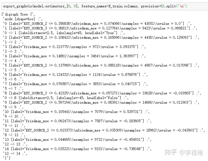
由于export_graphviz方法可以直接获取GBDT的树结构文本,所以可以对该文本进行解析,文本如下:
我自己写了个方法对这个树结构进行解析:
def get_gbdt_path(model, data_cols, char_cols=[], precision=6):
'''
根据数据集和GBDT模型,输出按照GBDT的路径衍生的变量:
------------------------------------------------------------
入参结果如下:
model: 训练完的GBDT模型
data_cols: 训练数据集的特征列表
char_cols: 类别特征的特征列表
由于类别特征需one-hot编码后进模型,在树结构中会出现var_value > 0.5的节点,传入char_cols则可以将节点改为var ==/!= value
precision: 提取每个子树的文字结构时,内部节点判断阈值的精确小数位,保留位数太少可能存在误差
------------------------------------------------------------
出参结果如下:
gbdt_path: GBDT所有叶子节点经过的路径
'''
# 类别特征节点判断转换的字段
if isinstance(char_cols, list) and char_cols != []:
node_judge_trans = {}
for char_col in char_cols:
for now_col in data_cols:
if char_col in now_col:
node_judge_trans['{} > 0.5'.format(now_col)] = '{} == {}'.format(char_col, now_col.replace(char_col + '_', ''))
node_judge_trans['{} <= 0.5'.format(now_col)] = '{} != {}'.format(char_col, now_col.replace(char_col + '_', ''))
# 所有树的叶子节点路径
leaf_node_path = []
# 遍历每棵子树
for n in range(model.n_estimators_):
tree_text = export_graphviz(model.estimators_[n, 0], feature_names=data_cols, precision=precision)
# 节点
node = {}
# 叶子节点
leaf_node_index = []
# 节点经过的路径
node_path = {}
# 分裂的节点
split_node = []
# 遍历每颗子树内部情况
for line in tree_text.split('n'):
# 获取现节点的索引
if '[label=' in line:
node_index = int(line[: line.find('[') - 1])
# 如果现节点有条件判断,保存判断
if 'label="friedman_mse' not in line:
node[node_index] = line[line.find('label="') + 7: line.find('nfriedman_mse')]
else:
leaf_node_index.append(node_index)
# 上一个节点到下一个节点的路径
if '->' in line:
# 获取上一个节点的索引
previous_node_index = int(line[: line.find('->') - 1])
# 获取下一个节点的索引
if '[' in line:
next_node_index = int(line[line.find('->') + 3: line.find('[') - 1])
else:
next_node_index = int(line[line.find('->') + 3: line.find(';') - 1])
# 分裂的左路径
if previous_node_index not in split_node:
split_node.append(previous_node_index)
# 从根节点到现节点的路径
if previous_node_index == 0:
node_path[next_node_index] = node[previous_node_index]
else:
node_path[next_node_index] = (node_path[previous_node_index] + ' & ' + node[previous_node_index])
# 分裂的右路径
else:
# 从根节点到现节点的路径
if previous_node_index == 0:
node_path[next_node_index] = node[previous_node_index].replace('<=', '>')
else:
node_path[next_node_index] = (node_path[previous_node_index] + ' & ' + node[previous_node_index].replace('<=', '>'))
if isinstance(char_cols, list) and char_cols != []:
# 遍历刚才生成的每个节点对应路径的字典
for index in node_path.keys():
# 由于类别特征会进行one-hot编码,导致节点的判断为<=0.5/>0.5,将其替换成未one-hot编码前的表达方式var ==/!= value
for old_judge, new_judge in node_judge_trans.items():
node_path[index] = node_path[index].replace(old_judge, new_judge)
leaf_node_path += [value for key, value in node_path.items() if key in leaf_node_index]
gbdt_path = {index + 1: value for index, value in enumerate(leaf_node_path)}
return gbdt_path运行该方法,得到gbdt_path:
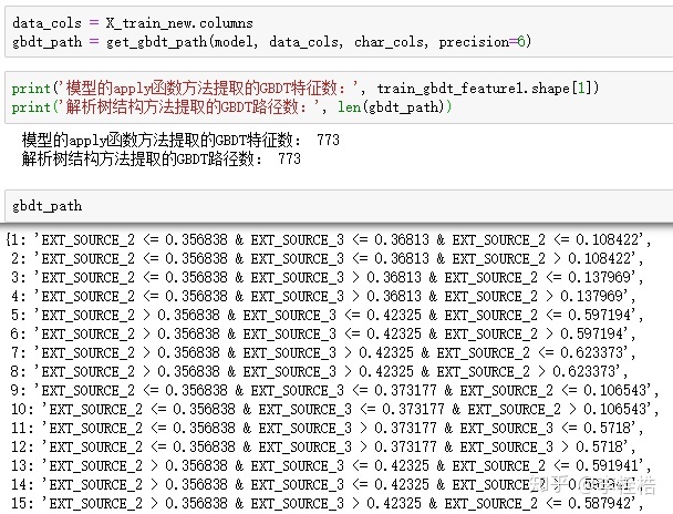
可以看到提取的GBDT路径有773条,也就是有773个叶子节点,数目等同于train_leaf_feature1的特征数。
接下来就可以对数据集根据GBDT的所有叶子节点经过的路径进行GBDT特征的提取,用下面的方法就可以直接提取:
def get_gbdt_feature(data, gbdt_path, cols_name=1):
'''
根据get_gbdt_path_var返回数据集的变量列表,回溯gbdt衍生给其他数据集:
------------------------------------------------------------
入参结果如下:
data: 需衍生变量的数据集,pd.DataFrame对象,不能有缺失
gbdt_cols: get_gbdt_path返回的GBDT所有叶子节点的对应路径
cols_name:是否使用GBDT路径作为列名,默认为1,传入0则将列名用叶子节点序号代替
------------------------------------------------------------
出参结果如下:
gbdt_feature: GBDT特征
'''
gbdt_feature = pd.DataFrame()
# 遍历所有叶子节点经过的路径提取GBDT特征
for key, value in gbdt_path.items():
# 需执行exec的字符串开头
if cols_name == 1:
exec_str = "gbdt_feature['{}'] = ".format(value)
elif cols_name == 0:
exec_str = "gbdt_feature['{}'] = ".format(key)
else:
raise ValueError('请传入正确的cols_name参数,cols_name应为1或0')
judge_len = len(value.split(' & '))
# 遍历变量名中的所有条件加到exec字符串中
for index, judge in enumerate(value.split(' & ')):
# 数值型的条件
if ('!=' not in judge) and ('==' not in judge):
# 只有一个条件
if judge_len == 1:
exec_str += ("(data['{}']{})".format(judge[: judge.find(' ')], judge[judge.find(' '):]))
# 第一个条件
elif index == 0:
exec_str += ("((data['{}']{})".format(judge[: judge.find(' ')], judge[judge.find(' '):]))
# 最后一个条件
elif index == judge_len - 1:
exec_str += (" & (data['{}']{}))".format(judge[: judge.find(' ')], judge[judge.find(' '):]))
# 中间的条件
else:
exec_str += (" & (data['{}']{})".format(judge[: judge.find(' ')], judge[judge.find(' '):]))
# 字符型的条件
else:
if '==' in judge:
offset = 3
else:
offset = 2
# 只有一个条件
if judge_len == 1:
exec_str += ("(data['{}']{}'{}')".format(judge[: judge.find(' ')],
judge[judge.find(' '): judge.find('=') + offset], judge[judge.find('=') + offset:]))
# 第一个条件
elif index == 0:
exec_str += ("((data['{}']{}'{}')".format(judge[: judge.find(' ')],
judge[judge.find(' '): judge.find('=') + offset], judge[judge.find('=') + offset:]))
# 最后一个条件
elif index == judge_len - 1:
exec_str += (" & (data['{}']{}'{}'))".format(judge[: judge.find(' ')],
judge[judge.find(' '): judge.find('=') + offset], judge[judge.find('=') + offset:]))
# 中间的条件
else:
exec_str += (" & (data['{}']{}'{}')".format(judge[: judge.find(' ')],
judge[judge.find(' '): judge.find('=') + offset], judge[judge.find('=') + offset:]))
# 将True/False替换成1/0
exec_str += ".astype(int)"
exec(exec_str)
return gbdt_feature提取结果如下:
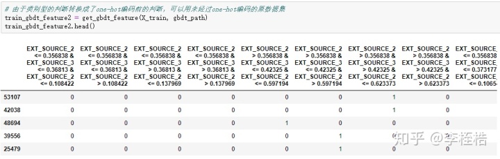
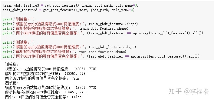
可以看到解析树结构提取的GBDT特征数比模型的apply函数提取的GBDT特征数少了28个,这是因为在不同的子树中存在相同的路径,所以用路径作为列名的时候,重复的路径只会在一列,相同的GBDT特征被去重了:

所以使用叶子节点的序号作为列名重新提取GBDT特征,这时候两个方法维度就相同了,并且解析树结构提取的GBDT特征与模型的apply函数提取的GBDT特征在训练集上完全相同,不过在测试集上出现了差异:
其实测试集上的差异因为使用export_graphviz获取GBDT的树结构文本时,节点判断条件的阈值按照precision参数保留了6个小数位,第45个叶子节点路径的最后一个判断条件保留成EXT_SOURCE_2 <= 0.591941,但是样本57072的EXT_SOURCE_2恰好为0.5919414304289855,所以就被划分到第46个叶子节点上了。
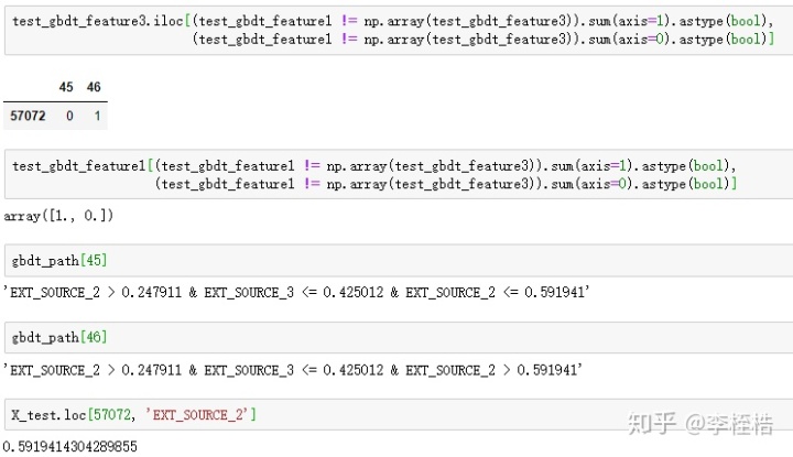
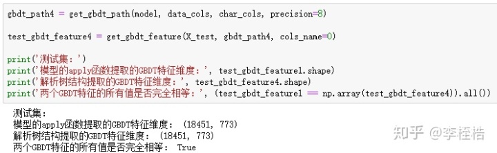
这里将get_gbdt_path的precision参数改为8,得到的测试集的新dGBDT特征就与模型的apply函数提取的GBDT特征完全相同了。
因为python的浮点型精度问题,其实如果precision设置太大也可能会出现误差,如果觉得误差可以接受,可以不去调整precision,一般误差的样本不多,都是特征值刚好卡在路径的条件判断阈值上的。
这样提取GBDT特征的方法还是很方便部署的,有了叶子节点经过的路径后,甚至可以直接在数据库里用sql语句去提取GBDT特征。
3. GBDT特征应用
GBDT特征一般与LR一起使用,将上面提取的GBDT直接作为LR的输入特征即可,这里就不详细说了。
我个人觉得GBDT特征是非常好的业务规则提取方法,可以使用GBDT快速提取叶子节点路径,如果路径符合业务解释则可以直接作为业务规则。而GBDT的几个参数,恰好可以调整规则的生成:
- max_depth:控制每条规则的最多使用特征个数,即一条规则的条件判断不超过max_depth个
- min_samples_leaf:控制每条规则的最少样本覆盖率,即一条规则的样本覆盖率不小于min_samples_leaf(float)
- n_estimators结合max_depth:控制规则个数,即提取的规则不超过n_estimators*2^(max_depth)个
用下面的代码提取覆盖率超过10%且使用特征在3个内的规则:
# 每条规则的最多使用3个特征,每条规则最少覆盖10%的样本,并且生成的规则个数不超过400个
model_rule = GradientBoostingClassifier(max_depth=3, min_samples_leaf=0.1, n_estimators=50, random_state=1234)
model_rule.fit(X_train_new, y_train)
gbdt_rule = get_gbdt_path(model_rule, data_cols, char_cols, precision=8)
train_gbdt_rule = get_gbdt_feature(X_train, gbdt_rule)
rule_df = pd.DataFrame(columns=['rule', 'cover', 'target'], index=range(train_gbdt_rule.shape[1]))
rule_df['rule'] = train_gbdt_rule.columns
data_count = len(y_train)
rule_df['cover'] = [round((train_gbdt_rule[rule] == 1).sum() / data_count, 4)
for rule in train_gbdt_rule.columns]
rule_df['target'] = [round(y_train[train_gbdt_rule[rule] == 1].sum() / (train_gbdt_rule[rule] == 1).sum(), 4)
for rule in train_gbdt_rule.columns]
rule_df = rule_df.sort_values('target', ascending=False)
rule_df.index = range(rule_df.shape[0])
print('总样本目标为 1 的样本占比为: {:.2f}%n'.format(100 * y_train.sum() / data_count))
print('根据目标占比,提取目标占比前 10 的规则,具体规则如下:')
for index in range(5):
print('>> 规则 {}: 覆盖率 {:.2f}% 目标占比 {:.2f}%'.format(index + 1, 100 * rule_df.loc[index, 'cover'], 100 * rule_df.loc[index, 'target']))
print(' {}n'.format(rule_df.loc[index, 'rule']))得到下面的结果:
总样本目标为 1 的样本占比为: 8.06%
根据目标占比,提取目标占比前 5 的规则,具体规则如下:
规则 1: 覆盖率 10.30% 目标占比 20.96% EXT_SOURCE_2 <= 0.3568377 & EXT_SOURCE_3 <= 0.36812986
规则 2: 覆盖率 11.61% 目标占比 20.22% EXT_SOURCE_3 <= 0.39019689 & EXT_SOURCE_2 <= 0.37501432
规则 3: 覆盖率 10.05% 目标占比 19.89% EXT_SOURCE_1 <= 0.42324439 & DAYS_BIRTH > -19935.5 & EXT_SOURCE_2 <= 0.28651884
规则 4: 覆盖率 12.61% 目标占比 19.43% EXT_SOURCE_2 <= 0.48394567 & EXT_SOURCE_3 <= 0.26575312
规则 5: 覆盖率 10.85% 目标占比 19.36% EXT_SOURCE_3 <= 0.26434812 & EXT_SOURCE_3 > -0.49973637
可以看到每一条规则的样本覆盖率均超过10%,并且最好的规则目标占比为平均目标占比的2.6倍。


 1929
1929

 被折叠的 条评论
为什么被折叠?
被折叠的 条评论
为什么被折叠?
 到【灌水乐园】发言


