labelencoder函数_Pytorch的损失函数Loss function接口介绍

1.损失函数简介

损失函数，又叫目标函数，用于计算真实值和预测值之间差异的函数，和优化器是编译一个神经网络模型的重要要素。 损失Loss必须是标量，因为向量无法比较大小（向量本身需要通过范数等标量来比较）。 损失函数一般分为4种，HingeLoss 0-1 损失函数，绝对值损失函数，平方损失函数，对数损失函数。

损失函数的本质

任何一个有负对数似然组成的损失都是定义在训练集上的经验分布和定义在模型上的概率分布之间的交叉熵。例如，均方误差是经验分布和高斯模型之间的交叉熵。

我们先定义预测值sample和目标值target，然后用不同的损失函数计算其损失值。

import torch
from torch.autograd import Variable
import torch.nn as nn
import torch.nn.functional as F
sample = Variable(torch.ones(2,2))
target = Variable(torch.tensor([[0,1],[2,3]]))

sample 的值为：tensor([[1., 1.], [1., 1.]])。

target 的值为：tensor([[0, 1], [2, 3]])。

2. 绝对值损失 L1 loss

2.1 nn.L1Loss

L1Loss 取预测值和真实值的绝对误差的平均数，用于回归。

criterion = nn.L1Loss(reduction='mean')
loss = criterion(sample, target)
print(loss)

结果是：1。 L1Loss还支持reduction=sum.

2.2 nn.SmoothL1Loss

SmoothL1Loss 也叫作 Huber Loss，误差在 (-1,1) 上是平方损失，其他情况是 L1 损失，应用于回归。

criterion = nn.SmoothL1Loss()
loss = criterion(sample, target)
print(loss)

最后结果是：0.625。

为什么用Huber loss?

平方损失L2的结果是算术均值无偏估计，L1损失函数的结果是中值无偏估计。

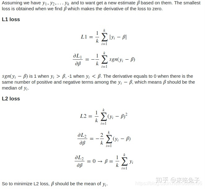
但是，平方损失容易被异常点影响。Huber loss 在0点附近是强凸，结合了平方损失和绝对值损失的优点。

3. 平方损失 MSE Loss

3.1 nn.MSELoss

平方损失函数，计算预测值和真实值之间的平方和的平均数，用于回归。

criterion = nn.MSELoss(reduction='mean')
loss = criterion(sample, target)
print(loss)

最后结果是：1.5。

4. 对数损失 -- 交叉熵

4.1 nn.CrossEntropyLoss

交叉熵损失函数，刻画的是实际输出（概率）与期望输出（概率）分布的距离，也就是交叉熵的值越小，两个概率分布就越接近。 CE loss用于分类。

CrossEntropyLoss类定义

import numpy as np
class CrossEntropyLoss():
    def __init__(self, weight=None, size_average=True):
        """
        初始化参数，因为要实现 torch.nn.CrossEntropyLoss 的两个比较重要的参数

        :param weight: 给予每个类别不同的权重
        :param size_average: 是否要对 loss 求平均
        """
        self.weight = weight
        self.size_average = size_average
    def __call__(self, input, target):
        """
        计算损失
        这个方法让类的实例表现的像函数一样，像函数一样可以调用

        :param input: (batch_size, C)，C是类别的总数
        :param target: (batch_size, 1)
        :return: 损失
        """
        batch_loss = 0.
        for i in range(input.shape[0]):
            numerator = np.exp(input[i, target[i]])     # 分子
            denominator = np.sum(np.exp(input[i, :]))   # 分母
            # 计算单个损失
            loss = -np.log(numerator / denominator)
            if self.weight:
                loss = self.weight[target[i]] * loss
            # 损失累加
            batch_loss += loss
        # 整个 batch 的总损失是否要求平均
        if self.size_average == True:
            batch_loss /= input.shape[0]
        return batch_loss

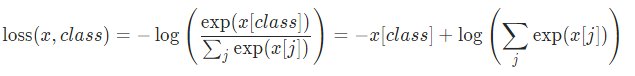
CE的公式是：

其中，

是不同类别的权重，默认为1.

需要注意的是，输入input要求为logit（模型输出且不经过softmax），target为该样本对应的类别, tensor long 类型（int64位）。

import torch 
sample = torch.tensor([[2.0,3],[1,3]])
target = torch.tensor([0,1])

criterion = nn.CrossEntropyLoss(reduction='mean')
loss = criterion(sample, target)
print(loss)

Output：tensor(0.7201)

上面CEloss的目标信息当做索引，与常见认识的交叉熵不太一样：

以下通过推导，证明CELoss和

两者是等价的。 使用 numpy来实现是这样的：

import numpy as np
def labelEncoder(y):
    nClass = max(y)+1
    tmp = np.zeros(shape = (y.shape[0], nClass))
    for i in range(y.shape[0]):
        tmp[i][y[i]] = 1
    return tmp
    
def softmax(x):
    print('exp',np.exp(x))
    print('sum',np.sum(np.exp(x),axis=1,keepdims=True))
    return np.exp(x)/np.sum(np.exp(x),axis=1,keepdims=True)
    
def crossEntropy(pred_logit, target):
    '''
    需要注意，这里只是计算一个样本的CE，如果样本数不为1，一般是需要除于样本数的.
    '''
    target = labelEncoder(target)
    pred = softmax(pred_logit)
    H = np.mean(np.sum(-target*np.log(pred),axis=1))
    return H
pred_logit = np.array([[2.0,3],[1,3]])
target = np.array([0,1])
H = crossEntropy(pred_logit, target)
print("H",H)

输出：

H 0.7200948492805976

对上了！ 再回头看看，公式

这里，就是class 就是索引，（调用 nn.CrossEntropyLoss需要注意），这里把Softmax求p 和 ylog(p)写在一起，一开始还没反应过来。

4.2 nn.BCELoss

二分类交叉熵把

当做两项分布，计算出来的loss就比交叉熵大（因为包含了正类和负类的交叉熵了）。 计算公式：

接口：torch.nn.BCELoss(weight=None, size_average=None, reduce=None, reduction='mean') BCE Loss类的定义：

class BCELoss(_WeightedLoss):
    r"""
    Examples::
        >>> m = nn.Sigmoid()
        >>> loss = nn.BCELoss()
        >>> input = torch.randn(3, requires_grad=True)
        >>> target = torch.empty(3).random_(2)
        >>> output = loss(m(input), target)
        >>> output.backward()
    """
    __constants__ = ['reduction', 'weight']

    def __init__(self, weight=None, size_average=None, reduce=None, reduction='mean'):
        super(BCELoss, self).__init__(weight, size_average, reduce, reduction)

    def forward(self, input, target):
        return F.binary_cross_entropy(input, target, weight=self.weight, reduction=self.reduction)

input输入为logit 经过sigmoid 后的值；target 是一个向量，并且向量元素取值0或1，这里不是 one-hot形式，具体理解是样本是否属于某个标签。比如，只有两类，target可以是[[1],[0]]，代表第一个样本是正类，第二个样本是反类，相应的input维度是(2,1)。target可以是[[1,0],[0,0]]，代表第一个样本属于第一个标签，不属于第二个标签，第二个样本既不属于第一个标签，也不属于第二个标签。

BCE 可以应用到多标签的分类任务中。 示例： 以二标签为例，即一个样本可以由两个标签。

sample = torch.tensor([[2.0,3.0],[1,3]])
target = torch.tensor([0,1])

one_hot_target = torch.zeros(target.shape[0], max(target)+1)
one_hot_target[torch.arange(target.shape[0]), target] = 1
sigmoid_input = torch.sigmoid(sample)
print('sigmoid_input',sigmoid_input)
print('one_hot_target',one_hot_target)

criterion = nn.BCELoss()
loss = criterion(sigmoid_input, one_hot_target)
print('bce',loss)

运行结果：

sigmoid_input:
 tensor([[0.8808, 0.9526],
        [0.7311, 0.9526]])
one_hot_target:
 tensor([[1., 0.],
        [0., 1.]])
bce tensor(1.1343)

人工计算： BCE Loss每个样本会进行取平均；最后，loss 还得处于样本数。

a = -(1*np.log(sigmoid_input[0][0]) + np.log(1-sigmoid_input[0][1]))/2
b = -(np.log(1-sigmoid_input[1][0]) + 1*np.log(sigmoid_input[1][1]))/2
print('cal bce',(a+b)/2)

结果：cal bce tensor(1.1343)

4.3 nn.NLLLoss

负对数似然损失函数（Negative Log Likelihood），也用于分类。 NLL loss 定义：

和 CrossEntropy Loss 相比，NLL loss需要输入的input 是 logit 经过LogSoftmax处理后的值，CE loss 输入是logit；两者的target 都是标量值。 LogSoftmax定义为:

示例：

# NLL loss
torch.manual_seed(0)
input = torch.randn(3, 5)
target = torch.tensor([1, 0, 4])
print("input", input)

m = nn.LogSoftmax(dim=1)
loss = nn.NLLLoss()
output = loss(m(input), target)
print("NLL loss", output)
# CE loss
loss = nn.CrossEntropyLoss()
output = loss(input, target)
print("CE loss", output)

结果：

input tensor([[ 1.5410, -0.2934, -2.1788,  0.5684, -1.0845],
        [-1.3986,  0.4033,  0.8380, -0.7193, -0.4033],
        [-0.5966,  0.1820, -0.8567,  1.1006, -1.0712]])
NLL loss tensor(2.7184)
CE loss tensor(2.7184)

NLL loss 和CE loss API只是 是否内置LogSoftmax的区别。 如果手动计算NLL loss:

def LogSoftmax(x):
    return torch.log(torch.exp(x)/torch.sum(torch.exp(x),axis=1,keepdims=True))
log_softmax_input = LogSoftmax(input)

print("cal NLL loss", -(log_softmax_input[0][target[0]] + 
log_softmax_input[1][target[1]] + log_softmax_input[2][target[2]])/3)

结果：cal NLL loss tensor(2.7184)

4.4 nn.NLLLoss2d

和上面类似，但是多了几个维度，一般用在图片上。

input, (N, C, H, W)
target, (N, H, W)

比如用全卷积网络做分类时，最后图片的每个点都会预测一个类别标签。

criterion = nn.NLLLoss2d()
loss = criterion(sample, target)
print(loss)

4.5 BCEWithLogitsLoss

BCEWithLogitsLoss 定义:

与 BCELoss相比，input x为模型输出logit，不需要经过sigmoid处理。两者的target t都是one-hot形式。 示例：

# BCELoss
sigmoid = nn.Sigmoid()
torch.manual_seed(0)
input = torch.randn(3,2)
torch.manual_seed(3)
# target one-hot type,such as tensor([0., 1.]).
target = torch.empty(3,2).random_(2)
sigmoid_input = sigmoid(input)
criterion = nn.BCELoss()
print('bce',criterion(sigmoid_input,target))

#BCE_logit Loss
criterion = nn.BCEWithLogitsLoss()
print('BCE_logit',criterion(input,target))

运行结果：

bce tensor(0.9232)
BCE_logit tensor(0.9232)

4.6 MultiLabelSoftMarginLoss

MultiLabelSoftMarginLoss 和 BCEWithLogitsLoss 效果是一样的。 为什么多标签的软边缘损失？ 因为，支持一个样本含有多个标签，比如target = [1,0,1]，代表该样本属于类别0和类别2.

# MultiLabelSoftMarginLoss
import torch 
from torch import nn
torch.manual_seed(0)
x = torch.randn(10, 3)
y = torch.FloatTensor(10, 3).random_(2)

bce_criterion = nn.BCEWithLogitsLoss(weight=None, reduce=False)
multi_criterion = nn.MultiLabelSoftMarginLoss(weight=None, reduce=False)

bce_loss = bce_criterion(x, y)
multi_loss = multi_criterion(x, y)

print('weight=None, bce_loss:n',torch.mean(bce_loss, dim = 1))
print('weight=None, multi_loss:n', multi_loss)

运行结果:

weight=None, bce_loss:
 tensor([1.1364, 0.8481, 1.2125, 0.5471, 0.5923, 0.7981, 0.9105, 0.4012, 0.5593,
        0.6012])
weight=None, multi_loss:
 tensor([1.1364, 0.8481, 1.2125, 0.5471, 0.5923, 0.7981, 0.9105, 0.4012, 0.5593,
        0.6012])

如果添加类的权重或者是每个样本添加权重:

#  the loss for class 1
class_weight = torch.FloatTensor([1.0, 2.0, 1.0])
#  the loss for last sample
element_weight = torch.FloatTensor([1.0]*9 + [2.0]).view(-1, 1)
element_weight = element_weight.repeat(1, 3)

bce_criterion_class = nn.BCEWithLogitsLoss(weight=class_weight, reduce=False)
multi_criterion_class = nn.MultiLabelSoftMarginLoss(weight=class_weight, reduce=False)
bce_criterion_element = nn.BCEWithLogitsLoss(weight=element_weight, reduce=False)
multi_criterion_element = nn.MultiLabelSoftMarginLoss(weight=element_weight, reduce=False)

bce_loss_class = bce_criterion_class(x, y)
multi_loss_class = multi_criterion_class(x, y)
bce_loss_element = bce_criterion_element(x, y)
multi_loss_element = multi_criterion_element(x, y)

print("class weight, BCE loss:n", torch.mean(bce_loss_class,dim=1))
print("class weight, multi loss:n",multi_loss_class)
print("element weight, BCE loss:n", torch.mean(bce_loss_element,dim=1))
print("element weight, multi loss:n",multi_loss_element)

运行结果：

class weight, BCE loss:
 tensor([1.6121, 1.2497, 1.9556, 0.7249, 0.6772, 1.1468, 1.1855, 0.5207, 0.6838,
        0.9306])
class weight, multi loss:
 tensor([1.6121, 1.2497, 1.9556, 0.7249, 0.6772, 1.1468, 1.1855, 0.5207, 0.6838,
        0.9306])
element weight, BCE loss:
 tensor([1.1364, 0.8481, 1.2125, 0.5471, 0.5923, 0.7981, 0.9105, 0.4012, 0.5593,
        1.2023])
element weight, multi loss:
 tensor([1.1364, 0.8481, 1.2125, 0.5471, 0.5923, 0.7981, 0.9105, 0.4012, 0.5593,
        1.2023])

拓展：TensorFlow与BCE对应的损失函数 pytorch的BCEWithLogitsLoss和TensorFlow的 sigmoid_cross_entropy_with_logits一样的效果。

# BCE
from torch import nn
bce_criterion = nn.BCEWithLogitsLoss(weight = None, reduce = False)
logits = torch.tensor([[12,3,2],[3,10,1],[1,2,5],
[4,6.5,1.2],[3,6,1]],dtype=torch.float64)
target = torch.tensor([[1,0,1],[0,1,0],[0,0,1],[1,1,0],
[0,1,0]],dtype=torch.float64)
print("BCE",bce_criterion(logits, target))
# sigmoid_cross_entropy_with_logits
import tensorflow as tf
sess =tf.Session()
sigmoid_CE = sess.run(tf.nn.sigmoid_cross_entropy_with_logits(logits=logits,labels=target))
print('sigmoid_CE',sigmoid_CE)

result：

BCE tensor([[6.1442e-06, 3.0486e+00, 1.2693e-01],
        [3.0486e+00, 4.5399e-05, 1.3133e+00],
        [1.3133e+00, 2.1269e+00, 6.7153e-03],
        [1.8150e-02, 1.5023e-03, 1.4633e+00],
        [3.0486e+00, 2.4757e-03, 1.3133e+00]], dtype=torch.float64)
sigmoid_CE [[6.14419348e-06 3.04858735e+00 1.26928011e-01]
 [3.04858735e+00 4.53988992e-05 1.31326169e+00]
 [1.31326169e+00 2.12692801e+00 6.71534849e-03]
 [1.81499279e-02 1.50231016e-03 1.46328247e+00]
 [3.04858735e+00 2.47568514e-03 1.31326169e+00]]

从结果来看，两个是等价的。

拓展：softmax_cross_entropy_with_logits

tensorflow 还有 softmax_cross_entropy_with_logits函数，以下比较它和 BCE Loss(这里用sigmoid_cross_entropy_with_logits 来实现)的区别：

# sigmoid_cross_entropy_with_logits
import tensorflow as tf
logits =tf.constant([[12,3,2],[3,10,1],[1,2,5],[4,6.5,1.2],[3,6,1]],dtype=tf.float64)
target = tf.constant([[1,0,1],[0,1,0],[0,0,1],[1,1,0],[0,1,0]],dtype=tf.float64)
sess =tf.Session()
sigmoid_CE = sess.run(tf.nn.sigmoid_cross_entropy_with_logits(logits=logits,
labels=target))
print('sigmoid_CE', np.mean(sigmoid_CE,axis=1))
# softmax CE with logits
softmax_CE = sess.run(tf.nn.softmax_cross_entropy_with_logits(
logits=logits,labels=target))
print("softmax_CE",softmax_CE)

运行结果：

sigmoid_CE [1.05850717 1.45396481 1.14896835 0.49431157 1.45477491]
softmax_CE [1.00003376e+01 1.03475622e-03 6.58839038e-02 2.66698414e+00
 5.49852354e-02]

两者结果不同，注意是一个对logit进行sigmoid操作；一个进行softmax操作。 Softmax运行原理：

def log_softmax(x):
    return -np.log(np.exp(x)/np.sum(np.exp(x),axis=1,keepdims=True))
logits = np.array([[12,3,2],[3,10,1],[1,2,5],[4,6.5,1.2],[3,6,1]])
target = np.array([[1,0,1],[0,1,0],[0,0,1],[1,1,0],[0,1,0]])
softmax_logit = log_softmax(logits)
loss = np.sum(softmax_logit*target,axis=1)
print("cal softmax loss",loss)

运行结果：

cal softmax loss [1.00003376e+01 1.03475622e-03 6.58839038e-02 2.66698414e+00
 5.49852354e-02]

---

参考：

1. Pytorch 论坛；
2. 图灵社区;
3. sshuair's notes PyTorch中的Loss Fucntion；
4. Difference of implementation between tensorflow softmax_cross_entropy_with_logits and sigmoid_cross_entropy_with_logits;
5. tf.nn.softmax_cross_entropy_with_logits的用法;
6. pytorch loss function，含 BCELoss;
7. 推荐！blog 交叉熵在神经网络的作用；
8. stack exchange Cross Entropy in network;
9. Cs231 softmax loss 与 cross entropy；
10. Pytorch nn.CrossEntropyLoss ;
11. NLLLoss 与CrossEntropyLoss区别 cnblog;
12. loss function 反向传播；
13. 书 deep learning 深度学习;
14. 机器学习中的损失函数(二) 回归问题的损失函数;