


文章目录
监督学习面临的基本挑战是:
- 需要多少数据才能合理地估计从输入到输出的未知的底层映射函数?
- 需要多少数据才能合理地估计近似映射函数的性能?
众所周知,通常情况下,训练数据太少会导致近似值不佳。过度约束的模型不足以拟合较小的训练数据集,而缺少约束的模型又可能会过拟合训练数据,两者均导致性能不佳。测试数据太少将导致对模型性能的高方差估计。
1. 数据集构建
作为探索的基础,使用一个简单的二分类来说明问题。
scikit-learn库提供了 make_circles() 函数,该函数可用于创建具有指定数量的样本和统计噪声的二进制分类问题。
每个示例都有两个输入变量,它们定义了二维平面上该点的x和y坐标。对于这两个类,这些点以两个同心圆排列(它们具有相同的中心)。
数据集中的点数由参数指定,其中每个圆将抽取一半。当通过定义噪声标准偏差的 noise 参数对点进行采样时,可以添加高斯噪声,其中0.0表示无噪声或从圆上精确绘制出的点。伪随机数生成器的种子可以通过 random_state 参数指定,该参数允许每次调用函数时都采样完全相同的点。
下面的示例从两个圆中生成100个无噪声且值为1的示例,以为伪随机数生成器提供种子。
from sklearn.datasets import make_circles
X, y = make_circles(n_samples=100, noise=0.0, random_state=1)
print(X.shape, y.shape)
for i in range(5):
	print(X[i], y[i])
输出:
(100, 2) (100,)
[-0.6472136 -0.4702282] 1
[-0.34062343 -0.72386164] 1
[-0.53582679 -0.84432793] 0
[-0.5831749  -0.54763768] 1
[ 0.50993919 -0.61641059] 1
可以看到输入变量的x和y分量以0.0为中心,并具有界限[-1,1]。类是0或1的整数,并且示例在各个类之间进行了shuffle。
1.1 构造正负类样本点
from sklearn.datasets import make_circles
from numpy import where
import matplotlib.pyplot as plt

X, y = make_circles(n_samples=100, noise=0.0, random_state=1)
zero_ix, one_ix = where(y == 0), where(y == 1)
plt.scatter(X[zero_ix, 0], X[zero_ix, 1], color='red')
plt.scatter(X[one_ix, 0], X[one_ix, 1], color='blue')
plt.show()
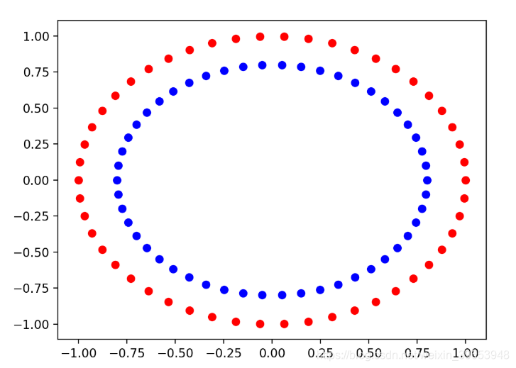
其中正类(1)为蓝色,负类(0)为红色。
1.2 添加噪声
所有真实数据都有统计噪声。统计噪声越大,意味着学习算法将输入变量映射到输出或目标变量的问题就越具有挑战性。nake_circles() 函数通过 noise 参数来模拟将噪声添加到样本中。
分别创建具有不同噪声的样本数据:
# scatter plots of the circles dataset with varied amounts of noise
from sklearn.datasets import make_circles
from numpy import where
import matplotlib.pyplot as plt

# create a scatter plot of the circles dataset with the given amount of noise
def scatter_plot_circles_problem(noise_value):
	# generate circles
	X, y = make_circles(n_samples=100, noise=noise_value, random_state=1)
	# select indices of points with each class label
	zero_ix, one_ix = where(y == 0), where(y == 1)
	# points for class zero
	plt.scatter(X[zero_ix, 0], X[zero_ix, 1], color='red')
	# points for class one
	plt.scatter(X[one_ix, 0], X[one_ix, 1], color='blue')

# vary noise and plot
values = [0.0, 0.1, 0.2, 0.3]
for i in range(len(values)):
	value = 220 + (i+1)
	plt.subplot(value)
	scatter_plot_circles_problem(values[i])
plt.show()
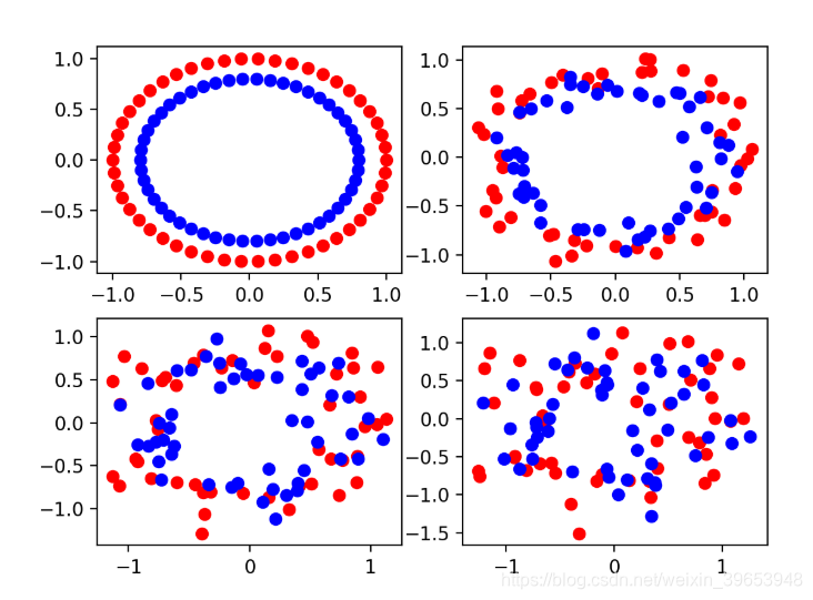
可以看到,少量的噪声0.1使该问题具有挑战性,但仍可区分。噪声值为0.0是不现实的,如此完美的数据集将不需要机器学习。0.2的噪声值使该问题非常具有挑战性,而0.3的噪声值可能使该问题难以学习。
1.3 增加样本数量
可以使用不同数量的样本来创建问题的相似图。更多的样本为学习算法提供了更多的机会来理解输入到输出的底层映射,进而获得性能更好的模型。
# scatter plots of the circles dataset with varied sample sizes
from sklearn.datasets import make_circles
from numpy import where
import matplotlib.pyplot as plt

# create a scatter plot of the circles problem
def scatter_plot_circles_problem(n_samples, noise_value=0.1):
	# generate circles
	X, y = make_circles(n_samples=n_samples, noise=noise_value, random_state=1)
	# select indices of points with each class label
	zero_ix, one_ix = where(y == 0), where(y == 1)
	# points for class zero
	plt.scatter(X[zero_ix, 0], X[zero_ix, 1], color='red')
	# points for class one
	plt.scatter(X[one_ix, 0], X[one_ix, 1], color='blue')

# vary sample size and plot
values = [50, 100, 500, 1000]
for i in range(len(values)):
	value = 220 + (i+1)
	plt.subplot(value)
	scatter_plot_circles_problem(values[i])
plt.show()
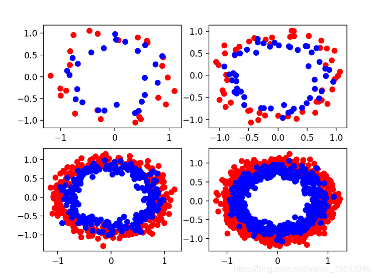
可以看到50个示例可能太少了,100个样本点看起来也不足以真正了解问题。该图表明,500和1,000个示例可能更容易学习,两个圆圈重叠掩盖了许多离群的点。
2. 神经网络模型的方差
使用Keras开发一个小的MLP模型,该模型有两个输入,隐藏层中的25个节点和一个输出。使用relu激活函数。由于是二分类问题,因此该模型可以在输出层上使用S型激活函数来预测属于0类或1类的样本的概率。使用Adam的小批量随机梯度下降的有效版本来训练模型,其中模型中的每个权重都有其自己的自适应学习率。二分类交叉熵损失函数作为优化函数,其中较小的损失值表示更好的模型拟合。
创建这些给定大小的训练集和测试集,并使用默认噪声0.1。完整代码如下:
from sklearn.datasets import make_circles
from keras.layers import Dense
from keras.models import Sequential

# create a test dataset
def create_dataset(n_train, n_test, noise=0.1):
	# generate samples
	n_samples = n_train + n_test
	X, y = make_circles(n_samples=n_samples, noise=noise, random_state=1)
	# split into train and test
	trainX, testX = X[:n_train, :], X[n_train:, :]
	trainy, testy = y[:n_train], y[n_train:]
	# return samples
	return trainX, trainy, testX, testy

# create dataset
trainX, trainy, testX, testy = create_dataset(500, 500)
# define model
model = Sequential()
model.add(Dense(25, input_dim=2, activation='relu'))
model.add(Dense(1, activation='sigmoid'))
model.compile(loss='binary_crossentropy', optimizer='adam', metrics=['accuracy'])
# fit model
history = model.fit(trainX, trainy, epochs=500, verbose=0)
# evaluate the model
_, test_acc = model.evaluate(testX, testy, verbose=0)
print('Test Accuracy: %.3f' % (test_acc*100))
在这种情况下,该模型的估计精度约为84.4%。
2.1 随机学习算法
每次运行示例时,数据集中的示例都是相同的。这是因为我们在创建样本时修复了伪随机数生成器。样本确实有噪声,但是每次都得到相同的噪声。
神经网络是一种非线性学习算法,这意味着它们可以学习输入变量和输出变量之间的复杂非线性关系。它们可以近似具有挑战性的非线性函数。
因此,将神经网络模型称为具有高方差低偏差的模型。它们具有较低的偏差,因为该方法很少对映射函数的数学函数形式进行假设。它们具有很大的差异,因为它们对用于训练模型的特定示例敏感。训练示例中的差异可能意味着生成的模型也非常不同,而技能又不同。
尽管神经网络是一种高方差低偏差方法,但是当在相同的生成的数据点上运行相同的算法时,这并不是造成估计性能差异的原因。
取而代之的是,由于学习算法是随机的,因此看到了多次运行的性能差异。
学习算法使用随机性元素来帮助模型在学习如何将输入变量映射到训练数据集中的输出变量的平均水平上做好工作。随机性的示例包括用于初始化模型权重的较小随机值,以及在每个训练时期之前对训练数据集中的示例进行随机排序。
这是有用的随机性,因为它允许模型自动“ 发现 ”映射功能的良好解决方案。令人沮丧的是,每次运行学习算法时,它通常会找到不同的解决方案,有时解决方案之间的差异很大,从而导致在对新数据进行预测时模型的估计性能有所不同。
2.2 平均模型性能
通过总结多次运行方法的性能,我们可以抵消特定神经网络发现的解决方案中的差异。
这涉及将同一算法多次拟合到同一数据集上,但允许每次运行算法时在学习算法中使用的随机性发生变化。每次运行都在相同的测试集上评估模型,并记录分数。在所有重复的末尾,使用均值和标准差汇总分数的分布。
模型在多次运行中的性能平均值给出了特定模型在特定数据集上的平均性能的概念。分数的分布或标准偏差给出了学习算法引入的方差的概念。
考虑到大数定律,更多的运行将意味着更准确的估计。为了使运行时间保持适度,重复运行10次。过boxplot函数使用盒形图和晶须图来总结分布。
# repeated evaluation of mlp on the circles dataset
from sklearn.datasets import make_circles
from keras.layers import Dense
from keras.models import Sequential
from numpy import mean
from numpy import std
import matplotlib.pyplot as plt

# create a test dataset
def create_dataset(n_train, n_test, noise=0.1):
	# generate samples
	n_samples = n_train + n_test
	X, y = make_circles(n_samples=n_samples, noise=noise, random_state=1)
	# split into train and test
	trainX, testX = X[:n_train, :], X[n_train:, :]
	trainy, testy = y[:n_train], y[n_train:]
	# return samples
	return trainX, trainy, testX, testy

# evaluate an mlp model
def evaluate_model(trainX, trainy, testX, testy):
	# define model
	model = Sequential()
	model.add(Dense(25, input_dim=2, activation='relu'))
	model.add(Dense(1, activation='sigmoid'))
	model.compile(loss='binary_crossentropy', optimizer='adam', metrics=['accuracy'])
	# fit model
	model.fit(trainX, trainy, epochs=500, verbose=0)
	# evaluate the model
	_, test_acc = model.evaluate(testX, testy, verbose=0)
	return test_acc

# create dataset
trainX, trainy, testX, testy = create_dataset(500, 500)
# evaluate model
n_repeats = 10
scores = list()
for i in range(n_repeats):
	# evaluate model
	score = evaluate_model(trainX, trainy, testX, testy)
	# store score
	scores.append(score)
	# summarize score for this run
	print('>%d: %.3f' % (i+1, score*100))
# report distribution of scores
mean_score, std_score = mean(scores)*100, std(scores)*100
print('Score Over %d Runs: %.3f (%.3f)' % (n_repeats, mean_score, std_score))
# plot distribution
plt.boxplot(scores)
plt.show()
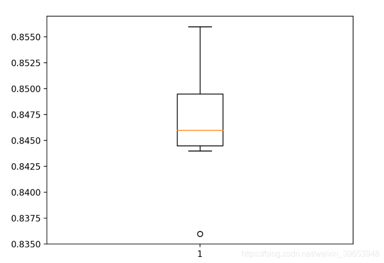
运行示例首先报告每个重复评估的模型得分。具体分数会有所不同,在此过程中,准确度分数介于83%和85%之间。在重复结束时,平均得分据报告约为84.7%,标准偏差约为0.5%。这意味着对于在特定训练集上进行训练并在特定测试集上进行评估的特定模型,假设与平均值存在三个标准偏差,则99%的运行将导致83.2%至86.2%的测试准确性。毫无疑问,样本数量很少(10个样本)导致了这些估计的误差。
创建了测试准确度分数的箱形图,显示了该框所表示的分数的中间50%(称为四分位数范围),范围从略低于84.5%到略低于85%。还可以看到,观察到的83%值可能是一个离群值(以点表示)。
2.3 数据集大小对测试准确率的影响
给定固定数量的含有噪声的数据集和具有合理配置的模型,模型拟合需要多大的数据集?可以通过评估适合不同大小的训练数据集的MLP模型的性能来研究该问题。
作为基础,可以定义大量示例,并认为这些示例足以解决该问题,例如100,000个,将其用作训练示例数量的上限,并在测试集中使用许多示例。定义一个在此数据集上表现良好的模型,作为已经有效学习了两个圆圈问题的模型。然后,通过对具有不同大小的训练数据集的模型进行拟合进行实验,并在测试集上评估其性能。
太少的示例将导致较低的测试准确性,这可能是因为所选模型过于适合训练集或训练集不足以代表问题。太多的示例将导致良好的测试精度,但可能会略低于理想的测试精度,这可能是因为所选模型没有能力学习这么大的训练数据集的细微差别,或者该数据集过分地代表了问题。训练数据集大小对模型测试精度的折线图应显示出增加的趋势,以至收益递减的点,甚至可能最终导致性能略有下降。
# study of training set size for an mlp on the circles problem
from sklearn.datasets import make_circles
from keras.layers import Dense
from keras.models import Sequential
from numpy import mean
from matplotlib import pyplot

# create train and test datasets
def create_dataset(n_train, n_test=100000, noise=0.1):
	# generate samples
	n_samples = n_train + n_test
	X, y = make_circles(n_samples=n_samples, noise=noise, random_state=1)
	# split into train and test, first n for test
	trainX, testX = X[n_test:, :], X[:n_test, :]
	trainy, testy = y[n_test:], y[:n_test]
	# return samples
	return trainX, trainy, testX, testy

# evaluate an mlp model
def evaluate_model(trainX, trainy, testX, testy):
	# define model
	model = Sequential()
	model.add(Dense(25, input_dim=2, activation='relu'))
	model.add(Dense(1, activation='sigmoid'))
	model.compile(loss='binary_crossentropy', optimizer='adam', metrics=['accuracy'])
	# fit model
	model.fit(trainX, trainy, epochs=500, verbose=0)
	# evaluate the model
	_, test_acc = model.evaluate(testX, testy, verbose=0)
	return test_acc

# repeated evaluation of mlp model with dataset of a given size
def evaluate_size(n_train, n_repeats=5):
	# create dataset
	trainX, trainy, testX, testy = create_dataset(n_train)
	# repeat evaluation of model with dataset
	scores = list()
	for _ in range(n_repeats):
		# evaluate model for size
		score = evaluate_model(trainX, trainy, testX, testy)
		scores.append(score)
	return scores

# define dataset sizes to evaluate
sizes = [100, 1000, 5000, 10000]
score_sets, means = list(), list()
for n_train in sizes:
	# repeated evaluate model with training set size
	scores = evaluate_size(n_train)
	score_sets.append(scores)
	# summarize score for size
	mean_score = mean(scores)
	means.append(mean_score)
	print('Train Size=%d, Test Accuracy %.3f' % (n_train, mean_score*100))
# summarize relationship of train size to test accuracy
pyplot.plot(sizes, means, marker='o')
pyplot.show()
# plot distributions of test accuracy for train size
pyplot.boxplot(score_sets, labels=sizes)
pyplot.show()
Train Size=100, Test Accuracy 72.041
Train Size=1000, Test Accuracy 83.719
Train Size=5000, Test Accuracy 84.062
Train Size=10000, Test Accuracy 84.025
随着训练集的增加,测试准确性的稳步提高。模型平均性能从5,000个示例到10,000个示例的过程中出现了下降,这很可能突出显示数据样本中的方差已超出所选模型配置(层和节点数)的容量。
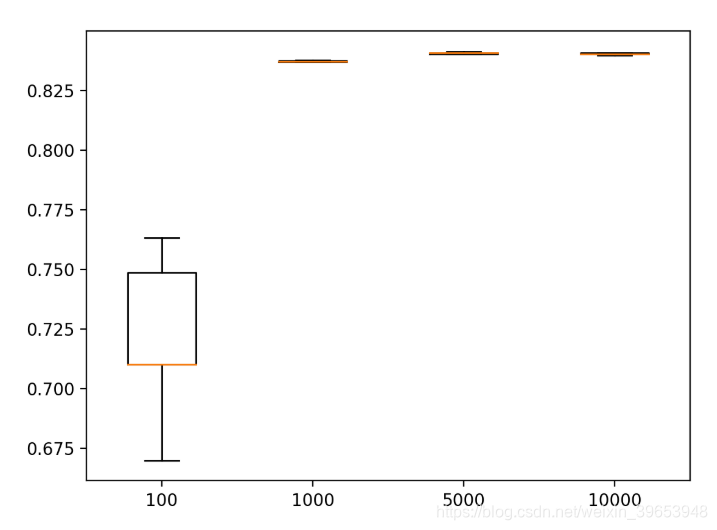
创建一个箱须图,显示每种尺寸的训练数据集的测试准确性得分的分布。正如预期的那样,我们可以看到,随着训练集大小的增加,测试集准确度分数的分布急剧减小,尽管在给定比例的情况下,该图的规模仍然很小。
2.4 测试集大小对测试精度的影响
在给定固定模型和固定训练数据集的情况下,需要多少测试数据才能准确估计模型性能?可以通过为MLP配置固定大小的训练集并使用不同大小的测试集评估模型来研究该问题。
使用与上一节中的研究几乎相同的策略。将训练集的大小固定为1,000个示例,因为它产生了一个相当有效的模型,当对100,000个示例进行评估时,估计的准确性约为83.7%。希望有一个较小的测试集大小可以合理地近似此值。
# study of test set size for an mlp on the circles problem
from sklearn.datasets import make_circles
from keras.layers import Dense
from keras.models import Sequential
from numpy import mean
from matplotlib import pyplot

# create dataset
def create_dataset(n_test, n_train=1000, noise=0.1):
	# generate samples
	n_samples = n_train + n_test
	X, y = make_circles(n_samples=n_samples, noise=noise, random_state=1)
	# split into train and test, first n for test
	trainX, testX = X[:n_train, :], X[n_train:, :]
	trainy, testy = y[:n_train], y[n_train:]
	# return samples
	return trainX, trainy, testX, testy

# fit an mlp model
def fit_model(trainX, trainy):
	# define model
	model = Sequential()
	model.add(Dense(25, input_dim=2, activation='relu'))
	model.add(Dense(1, activation='sigmoid'))
	model.compile(loss='binary_crossentropy', optimizer='adam', metrics=['accuracy'])
	# fit model
	model.fit(trainX, trainy, epochs=500, verbose=0)
	return model

# evaluate a test set of a given size on the fit models
def evaluate_test_set_size(models, n_test):
	# create dataset
	_, _, testX, testy = create_dataset(n_test)
	scores = list()
	for model in models:
		# evaluate the model
		_, test_acc = model.evaluate(testX, testy, verbose=0)
		scores.append(test_acc)
	return scores

# create fixed training dataset
trainX, trainy, _, _ = create_dataset(10)
# fit one model for each repeat
n_repeats = 10
models = [fit_model(trainX, trainy) for _ in range(n_repeats)]
print('Fit %d models' % n_repeats)
# define test set sizes to evaluate
sizes = [100, 1000, 5000, 10000]
score_sets, means = list(), list()
for n_test in sizes:
	# evaluate a test set of a given size on the models
	scores = evaluate_test_set_size(models, n_test)
	score_sets.append(scores)
	# summarize score for size
	mean_score = mean(scores)
	means.append(mean_score)
	print('Test Size=%d, Test Accuracy %.3f' % (n_test, mean_score*100))
# summarize relationship of test size to test accuracy
pyplot.plot(sizes, means, marker='o')
pyplot.show()
# plot distributions of test size to test accuracy
pyplot.boxplot(score_sets, labels=sizes)
pyplot.show()
输出:
Fit 10 models
Test Size=100, Test Accuracy 86.100
Test Size=1000, Test Accuracy 82.410
Test Size=5000, Test Accuracy 84.228
Test Size=10000, Test Accuracy 83.760
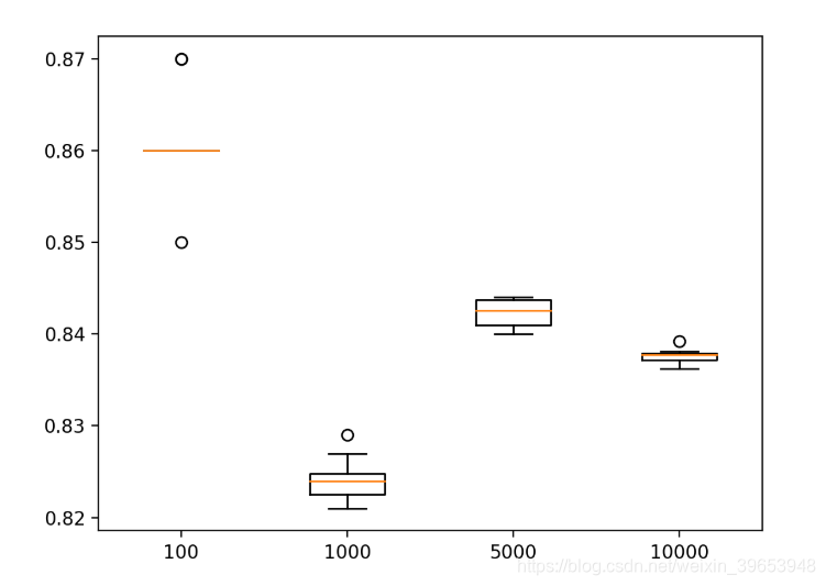
箱形图和晶须图显示,较小的测试集显示出分数的大范围分布。
上述内容没有针对从领域中抽取的随机示例报告所选模型的平均性能。该模型和示例是固定的,唯一的变化来源是来自学习算法。该研究表明,模型的估计准确性对测试数据集的大小有多敏感。这是一个重要的考虑因素,因为通常很少考虑测试集的大小,对于训练/测试集拆分,通常使用70%/ 30%或80%/ 20%的拆分。
参考:
https://machinelearningmastery.com/impact-of-dataset-size-on-deep-learning-model-skill-and-performance-estimates/


 9505
9505

 被折叠的 条评论
为什么被折叠?
被折叠的 条评论
为什么被折叠?
 到【灌水乐园】发言


