tensorflow loss到多少_[腾讯机智] tensorflow profiling工具简介——tensorflow原生工具

导语: 在使用tensorflow的过程中，我们经常需要使用工具来监测模型的运行性能。我们将通过一系列文章来介绍他们。本系列的前两篇文章主要介绍了nvidia提供的用于监测gpu的工具，本篇将介绍tensorflow原生的工具。

注意：

• 下面的示例默认为TF 2.0。
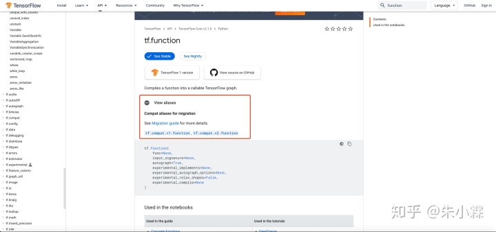
• 下面所有from tensorflow_core.python均为TF 2.0下使用方法，在TF.1x使用时请转为from tensorflow.python。
• 对于API函数在tf 1.x的兼容性名称，请在TF官方API文档中搜索，并点击词条中的"View Alias"来查看其兼容方法（如前缀为tf.compat.v1的API名称），如下图：

1 Timeline

Timeline主要描述了一个iteration GPU和CPU运行operation的时间过程。我们在进行模型调优的过程中经常需要通过Timeline数据来考查模型内部的实际运行情况。

1.1 生成Timeline

Timeline是通过 session 的运行时元数据 RunMetadata 得到的。所以我们需要在不同模型下操作 RunMetadata。

注意：

• 如果在生成是出现无法加载CUPTI，注意需要更新环境变量：

export LD_LIBRARY_PATH=/usr/local/cuda/extras/CUPTI/lib64:$LD_LIBRARY_PATH

加入后生成的tmeline中会出现gpu stream相关的信息，但是也会使timeline生成变大。并且实验中有出现tensorflow报错的情况，目前不能排除是个例。

下面便是不同API环境生成Timeline文件的方法：

1.1.1 Session (TF 1.x)

对于最传统的 Session 类模型，需要向 `sess.run` 中传入 `RunOptions` 和 `RunMetadata` 来获取元数据。

# 需要的import
from tensorflow_core.python.client import timeline
# 为了在TF 2.x中使用TF 1.x的功能，经常需要手动关闭eager execution
tf.compat.v1.disable_eager_execution()

# 需要传入run options才能返回得到run metadata
run_options = tf.compat.v1.RunOptions(trace_level=tf.compat.v1.RunOptions.FULL_TRACE)
run_metadata = tf.compat.v1.RunMetadata()

# 这里是构建模型的代码
# ...

# 在sess.run中加入run options和run metadata
sess.run(..., options=run_options, run_metadata=run_metadata)

# 运行结束后保存timeline
tl = timeline.Timeline(run_metadata.step_stats)
ctf = tl.generate_chrome_trace_format()
with open("timeline.json", 'w') as f:
    f.write(ctf)

1.1.2 Keras (TF 1.x & TF 2.x)

Keras取得 RunMetadata 的方式是在model.compile中加入。后续的步骤和 Session 一样。

# 需要的import
from tensorflow_core.python.client import timeline
# 为了在TF 2.x中使用TF 1.x的功能，经常需要手动关闭eager execution
tf.compat.v1.disable_eager_execution()

# 需要传入run options才能返回得到run metadata
run_options = tf.compat.v1.RunOptions(trace_level=tf.compat.v1.RunOptions.FULL_TRACE)
run_metadata = tf.compat.v1.RunMetadata()

# 这里是构建Keras模型的代码
# ...

# 在model.compile中加入run options和run metadata
model.compile(...,
              options=run_options, run_metadata=run_metadata)

model.fit(...)

# 运行后保存timeline
tl = timeline.Timeline(run_metadata.step_stats)
ctf = tl.generate_chrome_trace_format()
with open("timeline.json", 'w') as f:
    f.write(ctf)

1.1.3 Estimator (TF 1.x & TF 2.x)

Estimator 不能直接接触到 RunMetadata ，所以需要使用 ProfileHook。这个hook的文档在https://www.tensorflow.org/api_docs/python/tf/estimator/ProfilerHook

下面是一个例子，会按照步数在对应文件夹输出 timeline-x.json 文件。

# save_step指每多少步记录一次timeline。
hook = tf.estimator.ProfilerHook(save_steps=5, output_dir='tmp/')
estimator.train(
    input_fn=model_fn,
    hooks=[hook]
)

生成的Timeline文件会保存在 output_dir 参数中指示的位置，上面的例子中便是 tmp/。

1.2 查看Timeline

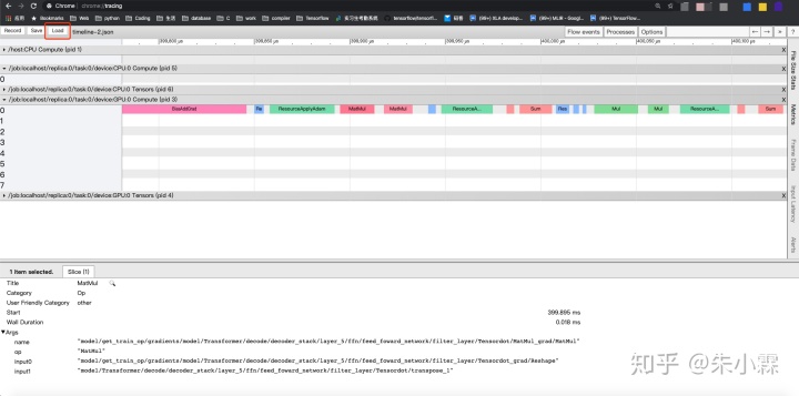
上面的方法均会输出类似timeline.json的文件，需要使用 Chrome Tracing Tool进行查看。在 Chrome 中打开 chrome://tracing 页面，点击 load 加载 json 文件。常用的控制方式是使用 W 和 S 进行放大和缩小， A 和 D 进行左右移动。

注意：

• 如果 Timeline 文件过大，可能会导致 Chrome 卡死。

查看结果的一个样例如下：

2 TensorBoard Profile (通过Tensorboard查看Timeline)

TensorBoard Profile 依托于 TensorBoard。TensorBoard 是 Tensorflow 配套的可视化工具。它功能非常丰富，可以用来追踪记录像 loss 和 accuracy 这样的实验数据，可视化模型的计算图等等。这一节介绍的 TensorBoard Profile 就是Tensorboard的众多功能之一，它类似于在 TensorBoard 中内嵌了 Timeline 信息，也就是一个 iteration 中 GPU 和 CPU 运行 op 的时间过程。这个记录 Timeline 的方法也是TF 2.x之后官方推荐的方法。关于TensorBoard Profile的官方介绍在这里：https://www.tensorflow.org/tensorboard/tensorboard_profiling_keras

2.1 生成Profile

针对 Tensorflow 的不同模型创建方法，有着不同的调用 TensorBoard 及 TensorBoard Profiling 的方法。在不同的TensorFlow API环境中，生成Profile的方法各不相同。下面分别介绍Keras和Eager API下生成Profile的方法。

2.1.1 Keras (TF 1.x & TF 2.x)

Keras 主要通过回调函数的方式使用 TensorBoard。具体为在 `model.fit` 中加入 TensorBoard 回调函数：

import tensorflow as tf

# 这里是制作keras模型的代码
# ...

log_dir="logs/profile/" + datetime.now().strftime("%Y%m%d-%H%M%S")
# 不含profile的一个tensorboard callback例子如下：
#  tensorboard_callback = tf.keras.callbacks.TensorBoard(log_dir=log_dir, histogram_freq=1)
# 包含profile的callback的例子如下：
# 这里profile_batch是profile第几个batch，0为关闭，默认为第二个。
tensorboard_callback = tf.keras.callbacks.TensorBoard(log_dir=log_dir, 
                                                      histogram_freq=1, 
                                                      profile_batch=3)
# 在model.fit中加入callback
model.fit(..., 
          callbacks=[tensorboard_callback])

代码中log_dir指定了TensorBoard整体信息的存储位置，Profile信息也会存在其中。

2.1.2 eager execution (TF2.x)

TF 2.x也可以不使用 Keras 构建模型，在这种情况下可以加入如下的代码来记录 TensorBoard Profile 信息。

# 需要添加的import
from tensorflow_core.python.eager import profiler

# 打开profiler
profiler.start()

# 这中间是训练相关的代码
# ...

# 关闭并保存
profiler_result = profiler.stop()
log_dir="logs/profile/" + datetime.now().strftime("%Y%m%d-%H%M%S")
profiler.save(log_dir, profiler_result)

和 Keras 的例子一样， log_dir指定了TensorBoard整体信息的存储位置，Profile信息也会存在其中。

这个方法经测试对 Keras 以及 TF 1.x 也都适用。

2.2 查看Profile

然后在对应位置（即上面例子中存储 logs/ 文件夹的位置）打开 TensorBoard 即可。打开方式为：

tensorboard --logdir=logs/

路径应设置为之前保存文件的最上层目录，也就是上面两个例子中的logs/。

启动TensorBoard后，到浏览器打开TensorBoard输出的本地接口（默认是 localhost:6006 ）进行查看

注意：

• 由于和普通 Timeline 一样，是通过 Chrome Tracing Tool 工作的，所以请使用 Chrome 浏览器。
• 目前即使在 Chrome 浏览器上使用也可能会出现问题，Profiling not showing up in Firefox 70 · Issue #2874 · tensorflow/tensorboard 。如果出现问题请退化回普通的 Timeline 生成方法。

3 tf.compat.v1.profiler 中的 profile 和 advise (TF 1.x & TF 2.x)

tf.compat.v1.profiler 曾经是 TF 1.x 的一个子模块 tfprof 。其中 profile 可以输出包含 timeline 在内的更多的信息（如 op 尺寸，计算量），而 advise 则是基于profile的结果输出部分优化建议。因为在使用中需要 RunMetadata，目前需要配合 Session 或者 Keras API 使用。

3.1 profile

添加如下代码可以生成profile信息：

# 这里是运行模型
# 注意如果需要时间或者内存信息，需要获取run metadata，获取方法在Timeline一节有提到
# ...

# 自定义profile设置
profile_opts = tf.compat.v1.profiler.profiler.ProfileOptionBuilder()  
                       # 选择监测的指标
                       .select(["bytes", "micros", "params", "float_ops"])  
                       # 输出文件，不设置则通过stdout在console输出
                       .with_file_output("profiler.txt") 
                       # 输出timeline
                       .with_timeline_output("timeline.json")
                       # 数据排序方式
                       .order_by("micros") 
                       # 通过build创建opts 
                       .build()

# 在默认图上运行profile
tf.compat.v1.profiler.profile(
    graph= tf.compat.v1.get_default_graph(),
    run_meta= run_metadata,  # 之前从模型中获得的run metadata
    cmd='op',
    options=profile_opts
)

更多示例请见：tensorflow/tensorflow

下面介绍常用参数：

• graph: 需要监测的图，基本上用 tf.get_default_graph() 就行了
• run_meta: 需要运行时相关的数据（如时间）时传入。Session模型和Keras模型取得 RunMetadata 的方法请见TImeline部分。
• cmd: 显示不同范围的数据，如op就是算子级别，注意op级别不能生成Timeline
• options: 用来控制输出的内容及位置等，一般可以直接用上面链接中的如tf.profiler.ProfileOptionBuilder.time_and_memory()这样的已经设置好的。也可以自定义，上面就是是一个自定义的例子。更多默认设置以及自定义方法请见：https://www.tensorflow.org/api_docs/python/tf/compat/v1/profiler/ProfileOptionBuilder 。

对于profile函数参数的更详细介绍请见https://www.tensorflow.org/api_docs/python/tf/compat/v1/profiler/profile

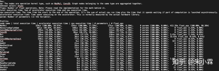
下面是profile输出的 profile.txt 的文件（在配置中 with_file_output(...) 中设置的文件名）的例子：

3.2 advise

advise信息通过下面代码获得它会给出一些优化建议。

# 上面是创建 session，运行并输出 run metadata 的代码
# ...

advice = tf.profiler.advise(sess.graph, run_meta=run_metadata)

示例输出如下：

ExpensiveOperationChecker:
top 1 operation type: MatMul, cpu: 172us, accelerator: 155us, total: 327us (10.94%)
top 2 operation type: Conv2DBackpropFilter, cpu: 164us, accelerator: 149us, total: 313us (10.47%)
top 3 operation type: ResourceApplyAdam, cpu: 142us, accelerator: 163us, total: 305us (10.20%)
top 1 graph node: gradients, cpu: 0us, accelerator: 0us, total: 0us
top 2 graph node: Adam, cpu: 1us, accelerator: 0us, total: 1us
top 3 graph node: fc1, cpu: 0us, accelerator: 0us, total: 0us


OperationChecker:
Found operation using NHWC data_format on GPU. Maybe NCHW is faster.

AcceleratorUtilizationChecker:
device: /job:localhost/replica:0/task:0/device:gpu:0 low utilization: 0.29

此输出为运行时的自动stdout输出，返回的 advice 是一个 AdviceProto 对象，其中存储了上面的console输出中的文本。

4 dump graph

在监测模型的过程中，我们往往希望观察模型的图以及节点上的属性。所以如何将图输出为文件供我们查看也很重要。

4.1 生成图文件

4.1.1 生成 TF graph (TF 1.x)

下面是一个输出图为 .pbtxt 文件的例子：

import tensorflow.compat.v1 as tf
tf.disable_eager_execution()

a = tf.add(1, 2, name="Add_these_numbers")
b = tf.multiply(a, 3)
c = tf.add(4, 5, name="And_These_ones")
d = tf.multiply(c, 6, name="Multiply_these_numbers")
e = tf.multiply(4, 5, name="B_add")
f = tf.div(c, 6, name="B_mul")
g = tf.add(b, d)
h = tf.multiply(g, f)

with tf.Session() as sess:
    tf.io.write_graph(sess.graph_def, "tmp", "graph.pbtxt")

这个例子会在 `tmp` 文件夹中输出 graph.pbtxt 文件。

4.1.2 XLA graph (TF 1.x & TF 2.x)

如果需要dump XLA的图，可以在运行时加入如下的flag

TF_XLA_FLAGS="--tf_xla_auto_jit=2 --tf_xla_clustering_debug" 
TF_DUMP_GRAPH_PREFIX="tmp/tf_graph" python3 mnist.py

其中 --tf_xla_auto_jit=2 是用来打开 XLA，--tf_xla_clustering_debug 用来打开 XLA 的 debug 模式，TF_DUMP_GRAPH_PREFIX 用来设置 XLA 相关的图的输出地址。默认会输出

• mark for compilation（xla中标注cluster的pass）前后的图，得到 before_mark_for_compilation_x.pbtxt mark_for_compilation_x.pbtxt mark_for_compilation_annotated_x.pbtxt
• increase dynamism for auto jit 前的图before_increase_dynamism_for_auto_jit_pass_x.pbtxt

上面的文件名均指一系列文件，其中x指其编号，推荐查看编号最大的一个。 这个例子是输出到 tmp/tf_graph 。 输出mark_for_compilation graph是由--tf_xla_clustering_debug 控制打开的

如果需要HLO相关的图可以设置flag为：

XLA_FLAGS="--xla_dump_to=tmp/hlo --xla_dump_hlo_as_html" 
TF_XLA_FLAGS="--tf_xla_auto_jit=2 --tf_xla_clustering_debug" python3 mnist.py

增加的flag XLA_FLAG 中的内容就是为输出HLO图的。上面的例子的输出地址为 tmp/hlo。

上述flag对应TF版本为TF 2.x，查看更多XLA flag请查看TensorFlow源码中的tensorflow/compiler/jit/flags.cc。

4.2 查看输出的图

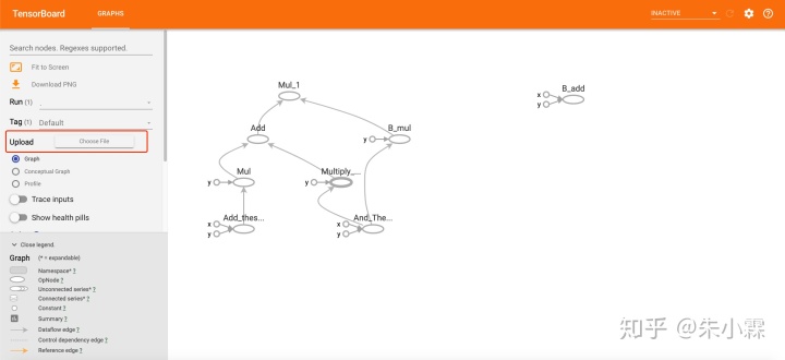
查看图需要使用 TensorBoard ，在 TensorBoard GRAPHS 部分的左侧点击Upload (Choose File)打开生成的 .pbtxt 文件查看图。XLA 的图会上面提及的 TF_DUMP_GRAPH_PREFIX flag 中设置的地址下。

上面的例子的示例如下：

对于HLO图，因为在flag中设置了输出为html，在 xla_dump_to 的flag设置的目录下直接查看生成的html文件。

5 后记

We're Hiring!

腾讯机器学习系统团队正在快速发展，诚邀各系统软件领域专业人士加盟。招聘方向包括但不限于机器学习框架（TensorFlow，PyTorch，MxNet等），编译器（LLVM，MLIR，XLA，Glow，TVM，PlaidML，Pluto等），GPU算子（CUDA，OpenCL等），分布式系统（Kubernetes，Spark等），AutoML（Ray，AutoKeras）。

简历投递xinanjiang@tencent.com