tensorflow lstm从隐状态到预测值_电商销售预测（3）--基于LSTM预测

最新推荐文章于 2024-03-28 17:49:09 发布

weixin_39793794

最新推荐文章于 2024-03-28 17:49:09 发布

阅读量700

点赞数 3

文章标签： tensorflow lstm从隐状态到预测值

前言

上文中我们采用lightgbm对销售数据进行了预测，对于lightgbm来说，特征工程很重要，尤其是特征与特征之间的关系。

对于时间序列来说，自身历史信息也很重要。而LSTM可以专门针对这种时间序列进行预测。因为他可以通过长短期记忆（long short term memory）来保留前一个时间步的cell状态。

对于LSTM，这里推荐两个英文博客，为啥是这两个？

因为几乎所有国内的翻译都找得到两个文章的影子。

Understanding LSTM Networkscolah.github.io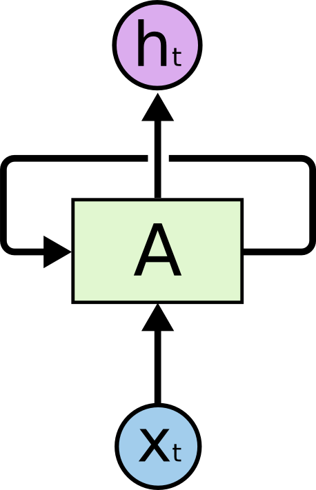

Multivariate Time Series Forecasting with LSTMs in Kerasmachinelearningmastery.com

至于中文版的，我之前参考过一处：

LSTM神经网络输入输出究竟是怎样的？www.zhihu.com

阅读本文你只需要了解的是：

LSTM 是一个神经网络，更具体是RNN （Recurrent ），所以我们需要用keras 基于tensorflow库
LSTM 相比于一般的神经网络（NN），增加了长时记忆与短时记忆。
LSTM 相比于一般的RNN，有效解决了梯度消失的问题。梯度消失通俗的影响就是“长期记忆的丢失”。
LSTM 相比于一般的RNN，从设计的角度来看，核心是多了一个cell。次核心是因为多了一个cell，每一步的迭代中重新设计了遗忘门，输入门和输出门，以及cell状态的更新。

okay，可以实战了。

准备数据

因为在前一篇文章中，我们已经分析过了这个数据集的基本情况。有兴趣的可以参考前两篇文章。

琥珀里有波罗的海：电商销售预测（1）--数据清理与融合zhuanlan.zhihu.com

琥珀里有波罗的海：电商销售预测（2）--特征工程与lightgbm预测zhuanlan.zhihu.com

所以我们会直接过渡到特征准备阶段，对于雷同的数据准备阶段，我们仅仅贴出代码。

首先是导入需要的库。

keras 是针对神经网络的库，这里我们的backend 是基于tensorflow的。因此这两个包都需要安装。

LSTM是属于keras的core layers，已经很好的封装，我们只需调用即可。训练神经网络，最好需要GPU，所以这里我采用google的notebook来操作。

import

读取数据部分。因为我们采用在线notebook，所以数据我也直接从kaggle上链接获取。

# read data
sales_train_file = '../input/competitive-data-science-predict-future-sales/sales_train.csv'
final_test_file = '../input/competitive-data-science-predict-future-sales/test.csv'
category_file = '../input/competitive-data-science-predict-future-sales/item_categories.csv'
item_file = '../input/competitive-data-science-predict-future-sales/items.csv'
shop_file = '../input/competitive-data-science-predict-future-sales/shops.csv'

一样的对时间基本处理：

item_all_df = pd.merge(item_df, category_df, on=['item_category_id'])
print(item_all_df.info())
# handle time data
dt_format = '%d.%m.%Y'
raw_df['date'] = pd.to_datetime(raw_df['date'], format=dt_format)
print(raw_df.head())
print(raw_df.info())

然后将每日的销售数据整理为每月的销售数据，并且将训练集扩展为商铺*商品的全矩阵。这部分的思路，请参考第一篇文章。

all_info_df = pd.merge(
    left=raw_df,
    right=item_all_df,
    on=['item_id'],
    how='left')
print(all_info_df.info())
all_info_df.drop(['item_name', 'item_category_name'], axis=1, inplace=True)
print(all_info_df.info())

# create time series period features
def time_period_features(df, time_col):
    # month level
    df['month'] = df[time_col].dt.month
    # quarter level
    df['quarter'] = df[time_col].dt.quarter
    # year level
    df['year'] = df[time_col].dt.year
    return df


all_info_df = time_period_features(all_info_df, 'date')
print(all_info_df.info())

sales_per_month = pd.pivot_table(
    data=all_info_df, values=[
        'item_cnt_day', 'item_price'], index=[
            'shop_id', 'item_id', 'item_category_id'], columns=[
                'year', 'month'], aggfunc={
                    'item_cnt_day': 'sum', 'item_price': 'mean'})
print(sales_per_month.info())


sales_per_month.fillna(0, inplace=True)
sales_per_month.reset_index(inplace=True)
print(sales_per_month.info())



for col in list(sales_per_month.columns)[3:]:
    sales_per_month[col] = sales_per_month[col].astype(np.float32)
print(sales_per_month.info())

# sales_per_month = pd.merge(left=sales_per_month, right=final_test_df[[
# #                            'shop_id', 'item_id']], on=['shop_id', 'item_id'], how='outer')

full_shop_item_matrix = pd.DataFrame([])
all_items = item_df[['item_id']]
for shop_id in shop_df['shop_id'].values:
    all_items_per_shop = all_items.copy()
    all_items_per_shop['shop_id'] = shop_id
    if full_shop_item_matrix.shape[0] ==0:
        full_shop_item_matrix = all_items_per_shop
    else:
        full_shop_item_matrix = pd.concat([full_shop_item_matrix, all_items_per_shop], axis=0)

print(full_shop_item_matrix.shape)

sales_per_month = pd.merge(left=sales_per_month,right= full_shop_item_matrix,on=['shop_id','item_id'],how='right')

print(sales_per_month.info())
sales_per_month.drop([('item_category_id', '', '')], axis=1, inplace=True)

sales_per_month = pd.merge(left=sales_per_month,
                           right=item_df[['item_id',
                                          'item_category_id']],
                           left_on=[('item_id',
                                     '',
                                     '')],
                           right_on=['item_id'],
                           how='right')

sales_per_month[('item_category_id', '', '')
                ] = sales_per_month['item_category_id']
sales_per_month.drop(['item_category_id', 'item_id'], inplace=True, axis=1)
print(sales_per_month.info())




sales_per_month.fillna(value=0, inplace=True)

print(sales_per_month.info())

到目前整理的结果如下：

<class 'pandas.core.frame.DataFrame'>
Int64Index: 1330200 entries, 0 to 1330199
Data columns (total 71 columns):
 #   Column                    Non-Null Count    Dtype  
---  ------                    --------------    -----  
 0   (shop_id, , )             1330200 non-null  int64  
 1   (item_id, , )             1330200 non-null  int64  
 2   (item_cnt_day, 2013, 1)   1330200 non-null  float32
 3   (item_cnt_day, 2013, 2)   1330200 non-null  float32
 4   (item_cnt_day, 2013, 3)   1330200 non-null  float32
 5   (item_cnt_day, 2013, 4)   1330200 non-null  float32
 6   (item_cnt_day, 2013, 5)   1330200 non-null  float32
 7   (item_cnt_day, 2013, 6)   1330200 non-null  float32
 8   (item_cnt_day, 2013, 7)   1330200 non-null  float32
 9   (item_cnt_day, 2013, 8)   1330200 non-null  float32
 10  (item_cnt_day, 2013, 9)   1330200 non-null  float32
 11  (item_cnt_day, 2013, 10)  1330200 non-null  float32
 12  (item_cnt_day, 2013, 11)  1330200 non-null  float32
 13  (item_cnt_day, 2013, 12)  1330200 non-null  float32
 14  (item_cnt_day, 2014, 1)   1330200 non-null  float32
 15  (item_cnt_day, 2014, 2)   1330200 non-null  float32
 16  (item_cnt_day, 2014, 3)   1330200 non-null  float32
 17  (item_cnt_day, 2014, 4)   1330200 non-null  float32
 18  (item_cnt_day, 2014, 5)   1330200 non-null  float32
 19  (item_cnt_day, 2014, 6)   1330200 non-null  float32
 20  (item_cnt_day, 2014, 7)   1330200 non-null  float32
 21  (item_cnt_day, 2014, 8)   1330200 non-null  float32
 22  (item_cnt_day, 2014, 9)   1330200 non-null  float32
 23  (item_cnt_day, 2014, 10)  1330200 non-null  float32
 24  (item_cnt_day, 2014, 11)  1330200 non-null  float32
 25  (item_cnt_day, 2014, 12)  1330200 non-null  float32
 26  (item_cnt_day, 2015, 1)   1330200 non-null  float32
 27  (item_cnt_day, 2015, 2)   1330200 non-null  float32
 28  (item_cnt_day, 2015, 3)   1330200 non-null  float32
 29  (item_cnt_day, 2015, 4)   1330200 non-null  float32
 30  (item_cnt_day, 2015, 5)   1330200 non-null  float32
 31  (item_cnt_day, 2015, 6)   1330200 non-null  float32
 32  (item_cnt_day, 2015, 7)   1330200 non-null  float32
 33  (item_cnt_day, 2015, 8)   1330200 non-null  float32
 34  (item_cnt_day, 2015, 9)   1330200 non-null  float32
 35  (item_cnt_day, 2015, 10)  1330200 non-null  float32
 36  (item_price, 2013, 1)     1330200 non-null  float32
 37  (item_price, 2013, 2)     1330200 non-null  float32
 38  (item_price, 2013, 3)     1330200 non-null  float32
 39  (item_price, 2013, 4)     1330200 non-null  float32
 40  (item_price, 2013, 5)     1330200 non-null  float32
 41  (item_price, 2013, 6)     1330200 non-null  float32
 42  (item_price, 2013, 7)     1330200 non-null  float32
 43  (item_price, 2013, 8)     1330200 non-null  float32
 44  (item_price, 2013, 9)     1330200 non-null  float32
 45  (item_price, 2013, 10)    1330200 non-null  float32
 46  (item_price, 2013, 11)    1330200 non-null  float32
 47  (item_price, 2013, 12)    1330200 non-null  float32
 48  (item_price, 2014, 1)     1330200 non-null  float32
 49  (item_price, 2014, 2)     1330200 non-null  float32
 50  (item_price, 2014, 3)     1330200 non-null  float32
 51  (item_price, 2014, 4)     1330200 non-null  float32
 52  (item_price, 2014, 5)     1330200 non-null  float32
 53  (item_price, 2014, 6)     1330200 non-null  float32
 54  (item_price, 2014, 7)     1330200 non-null  float32
 55  (item_price, 2014, 8)     1330200 non-null  float32
 56  (item_price, 2014, 9)     1330200 non-null  float32
 57  (item_price, 2014, 10)    1330200 non-null  float32
 58  (item_price, 2014, 11)    1330200 non-null  float32
 59  (item_price, 2014, 12)    1330200 non-null  float32
 60  (item_price, 2015, 1)     1330200 non-null  float32
 61  (item_price, 2015, 2)     1330200 non-null  float32
 62  (item_price, 2015, 3)     1330200 non-null  float32
 63  (item_price, 2015, 4)     1330200 non-null  float32
 64  (item_price, 2015, 5)     1330200 non-null  float32
 65  (item_price, 2015, 6)     1330200 non-null  float32
 66  (item_price, 2015, 7)     1330200 non-null  float32
 67  (item_price, 2015, 8)     1330200 non-null  float32
 68  (item_price, 2015, 9)     1330200 non-null  float32
 69  (item_price, 2015, 10)    1330200 non-null  float32
 70  (item_category_id, , )    1330200 non-null  int64  
dtypes: float32(68), int64(3)
memory usage: 385.6 MB
None

特征整理为3D数组

针对lightgbm我们添加了一些统计特征以及销售额的特征计算。

对于LSTM我们舍去这两种特征计算，主要是因为：

统计特征是过去月份的统计信息，（比如均值），可以通过函数来拟合。对于神经网络来说，这个不是特别难的事，没有必要显式的创造该特征
销售额也是已有特征的一个拟合，所以我们不会进行显式的计算
另外还有一个原因是该数据集占用内存较大，这里我们不会考虑过多的特征

对于LSTM的训练我们需要进一步整理数据集，因为keras的LSTM layer 接收的数据格式为3D数组，维度分别为：（样本数，时间步，特征个数)。

对于该案例：

假如我们只考虑历史价格和历史销售作为特征，我们的特征数就是2
假如我们考虑用过去18个月的数据作为一组数据，我们的时间步就是18
剩下的我们迭代的数据

对于输入和输出更多的了解，可以参考该链接。


# format the features
# use past 1 year data to predict
melt_data = pd.DataFrame([])  # 创建空df
feature_start_index = 2 # 跳过shop id 和item id
feature_loop_index = 18 # 选取过去18个月信息
one_catgory_feature_num = 34 #每个特征有34 个月信息
train_months = 33 



for i in range(one_catgory_feature_num - feature_loop_index):
    sales = sales_per_month.iloc[:, feature_start_index +
                                 i:feature_start_index + feature_loop_index + i] # 选取18个月的sales
    target = sales_per_month.iloc[:, feature_loop_index + i + 1] #下一个月为target
    target.name='target'
    sales.columns = [f'sales{i}' for i in range(feature_loop_index)]
    price = sales_per_month.iloc[:, feature_start_index +
                                    i +
                                    one_catgory_feature_num:feature_start_index +
                                                            feature_loop_index +
                                                            i +
                                                            one_catgory_feature_num] # 同理选取18个月的price
    price.columns = [f'price_{i}' for i in range(feature_loop_index)]
    sample = pd.concat([sales,price, target], axis=1)

    if i == 0:
        melt_data = sample
    else:

        melt_data = pd.concat([melt_data, sample], axis=0) # 按行合并

all_cols = [[f'price_{i}',f'sales_{i}'] for i in range(feature_loop_index)]
all_cols.append(['target'])
all_cols = sum(all_cols,[])

melt_data= melt_data[all_cols]  # reorder columns


print(sales.shape)
print(melt_data.shape[0])
print(one_catgory_feature_num - feature_loop_index)
one_set_num = int(melt_data.shape[0]/(one_catgory_feature_num - feature_loop_index)) # 每一组样本包含所有的商铺*商商品
melt_train_X = melt_data.iloc[0:one_set_num*(one_catgory_feature_num - feature_loop_index-1), :-1] # 取18*2 列作为特征
melt_train_y = melt_data.iloc[0:one_set_num*(one_catgory_feature_num - feature_loop_index-1), -1] # 最后一列是target
melt_validate_X = melt_data.iloc[one_set_num*(one_catgory_feature_num - feature_loop_index-1):, :-1] # 最后一组组为验证
melt_validate_y = melt_data.iloc[one_set_num*(one_catgory_feature_num - feature_loop_index-1):, -1]

# 同理做出test data
sales = sales_per_month.iloc[:, feature_start_index +
                             one_catgory_feature_num -
                             feature_loop_index:feature_start_index +
                             one_catgory_feature_num]
sales.columns = [f'sales_{i}' for i in range(feature_loop_index)]

price = sales_per_month.iloc[:, feature_start_index +
                             one_catgory_feature_num +
                             one_catgory_feature_num -
                             feature_loop_index:feature_start_index +
                             one_catgory_feature_num +
                             one_catgory_feature_num]
price.columns = [f'price_{i}' for i in range(feature_loop_index)]
melta_test_X = pd.concat([sales,price], axis=1)
all_cols = [[f'price_{i}',f'sales_{i}'] for i in range(feature_loop_index)]
all_cols = sum(all_cols,[])
melta_test_X = melta_test_X [all_cols]  # reorder columns

print(melt_train_X.shape)
print(melt_train_y.shape)
print(melt_validate_X.shape)
print(melt_validate_y.shape)
print(melta_test_X.shape)
shop_item_id = sales_per_month[[('shop_id','',''),('item_id','','')]]
shop_item_id.columns = ['shop_id','item_id'] # 将multiindex 改名


scaler = MinMaxScaler()
melt_train_X = scaler.fit_transform(melt_train_X)
melt_validate_X = scaler.transform(melt_validate_X)
melta_test_X = scaler.transform(melta_test_X)

# y_scaler = MinMaxScaler()
# 将数据转换为3D
# melt_train_y = y_scaler.fit_transform(melt_train_y.values.reshape(melt_train_y.shape[0],1))
# melt_train_y.reshape(melt_train_y.shape[0])
# melt_validate_y = y_scaler.transform(melt_validate_y.values.reshape(melt_train_y.shape[0],1))
# melt_validate_y.reshape(melt_validate_y.shape[0])

melt_train_X  = melt_train_X.reshape(melt_train_X.shape[0],int(melt_train_X.shape[1]/2),2)
melt_validate_X  = melt_validate_X.reshape(melt_validate_X.shape[0],int(melt_validate_X.shape[1]/2),2)
melta_test_X  = melta_test_X.reshape(melta_test_X.shape[0],int(melta_test_X.shape[1]/2),2)

fig,ax = plt.subplots(2,1)
ax[0].hist(melt_train_y)
ax[1].hist(melt_validate_y)
plt.show()

print(melt_train_X.shape)

在上述的代码中，我们做了以下变换：

提取18个月的销售数据和价格数据，作为一组样本
依次滚动迭代，取完33个月数据，每次创建一组样本
将所有的样本组融合成一个大样本（按行堆叠）
将price 和sales 重新调整顺序
切分训练组和验证组，测试组
对训练组和验证组进行归一化
将训练组和验证组，测试组转成3D数组

可以看到训练组的数据结构如下：1995万条样本，18个时间步，2个特征

(19953000, 18, 2)

建立LSTM模型

LSTM layer 是keras里面的核心layer，它的使用方法和一般的Dense layer 基本类似。主要的区分点在于以下几点：

input_shape： LSTM需要输入3D数组，我们一般输入(n_steps, n_features)，表面是2维，其实表示第1维（样本数量维）为None，也就是不做限制。
return_sequences：这个参数表示是否返回每一个时间步的隐藏特征（一般用h表示）。作为第一层输入，和中间层，会选择返回为True。最后一层LSTM 选择为False，表示只返回最后一步的隐藏特征
剩下的其他参数可以参考一般Dense层。

为了防止过拟合，我这里启动了dropout 比例。

n_hidenlayers = 5
dp_ratio = 0.4

n_steps = 18
n_features = 2
model = Sequential()
model.add(LSTM(16, dropout = dp_ratio,return_sequences=True, input_shape=(n_steps, n_features)))

#model.add(LSTM(n_hidenfreature, dropout = dp_ratio,return_sequences=False, input_shape=(n_hours, n_features)))

for _ in range(n_hidenlayers):
    model.add(LSTM(16,dropout = dp_ratio,return_sequences=True))

model.add(LSTM(8,dropout = dp_ratio))
model.add(Dense(1))
model.compile(loss='mse', optimizer='adam')
model.summary()


# Set callback functions to early stop training and save the best model so far
callbacks = [EarlyStopping(monitor='val_loss', patience=20),
             ModelCheckpoint(filepath='best_model.h5', monitor='val_loss', save_best_only=True)]

# fit network
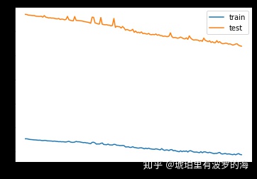
history = model.fit(melt_train_X, melt_train_y, epochs=150, batch_size=13302*5, callbacks = callbacks,validation_data=(melt_validate_X, melt_validate_y), verbose=1, shuffle=False)
# plot history
plt.plot(history.history['loss'], label='train')
plt.plot(history.history['val_loss'], label='test')
plt.legend()
plt.show()

建立好模型，我们可以预览一下模型的结构。可以注意到output shape里面的前5层的第二维都是18，表明我们返回sequence。最后一个LSTM 没有返回sequence，只返回最后一个时间步的隐藏状态。

Model: "sequential_1"
_________________________________________________________________
Layer (type)                 Output Shape              Param #   
=================================================================
lstm_1 (LSTM)                (None, 18, 16)            1216      
_________________________________________________________________
lstm_2 (LSTM)                (None, 18, 16)            2112      
_________________________________________________________________
lstm_3 (LSTM)                (None, 18, 16)            2112      
_________________________________________________________________
lstm_4 (LSTM)                (None, 18, 16)            2112      
_________________________________________________________________
lstm_5 (LSTM)                (None, 18, 16)            2112      
_________________________________________________________________
lstm_6 (LSTM)                (None, 18, 16)            2112      
_________________________________________________________________
lstm_7 (LSTM)                (None, 8)                 800       
_________________________________________________________________
dense_1 (Dense)              (None, 1)                 9         
=================================================================
Total params: 12,585
Trainable params: 12,585
Non-trainable params: 0

训练很漫长，因为我们的数据量达到了千万级别，16G内存+GPU的情况下，需要训练5个小时。

预测测试集

这里代码和上篇几乎一致，我们仅仅贴出代码。思路主要是：

预测全矩阵的下一个月销售
筛选出测试集中出现的组合
提交结果

result = shop_item_id.copy()
yhat = model.predict(melta_test_X)
result['item_cnt_month'] = yhat
# melt_test_df.reset_index(inplace=True)
result['item_cnt_month'].plot()
print(result.info())
result = pd.merge(
    final_test_df,
    result,
    left_on=[
        'shop_id',
        'item_id'],
    right_on=[
        'shop_id',
        'item_id'],
    how='left')
print(result.isna().any())
print(result.info())
# result.fillna(0, inplace=True)
# result['ID'] = result.index
result['item_cnt_month'].clip(0,20,inplace=True)

result[['ID', 'item_cnt_month']].to_csv('submission.csv', index=False)

总结

本文主要是通过LSTM来预测同该电商下一个月的销售情况。

LSTM 难点主要在于：

3维数据格式的构造
LSTM 模型参数的理解，尤其是input_shape以及return_sequence
LSTM 模型训练耗时

我对比了同一个数据集的两种模型的预测结果，lightgbm 速度快，精度相比于来说要要高，我提交的结果预测误差在1 以下，LSTM预测的结果误差比1略高。

后续如果模型参数有优化，我会继续更新到本文。

weixin_39793794

关注

3
点赞
踩
7

收藏

觉得还不错? 一键收藏
0
评论
tensorflow lstm从隐状态到预测值_电商销售预测（3）--基于LSTM预测

前言上文中我们采用lightgbm对销售数据进行了预测，对于lightgbm来说，特征工程很重要，尤其是特征与特征之间的关系。对于时间序列来说，自身历史信息也很重要。而LSTM可以专门针对这种时间序列进行预测。因为他可以通过长短期记忆（long short term memory）来保留前一个时间步的cell状态。对于LSTM，这里推荐两个英文博客，为啥是这两个？因为几乎所有国内的翻译都找得到两个...
复制链接

扫一扫