TensorFlow2.0 ANN实例之回归预测广告与销量

综述

通过使用Tf.keras.Sequential搭建实现非线性回归的神经网络模型。并理解针对问题空间如何设计网络结构，以及网络结构涉及到的优化器、损失函数的选择，回调函数的使用。完整数据与代码可在我的GitHub中下载。

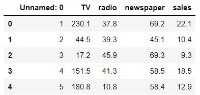
部分数据展示

TV	radio	newspaper	sales
230.1	37.8	69.2	22.1
44.5	39.3	45.1	10.4
17.2	45.9	69.3	9.3
151.5	41.3	58.5	18.5
180.8		10.8	58.4

代码

# 导入库
import tensorflow as tf
import numpy as np
import pandas as pd
import matplotlib as mpl
import matplotlib.pyplot as plt
%matplotlib inline

# 读入数据
data = pd.read_csv('Advertising.csv')
# 查看前五行数据
print(data.head())

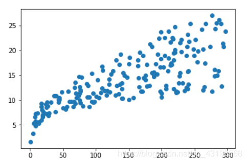
# 数据内容可视化
plt.scatter(data.TV, data.sales)
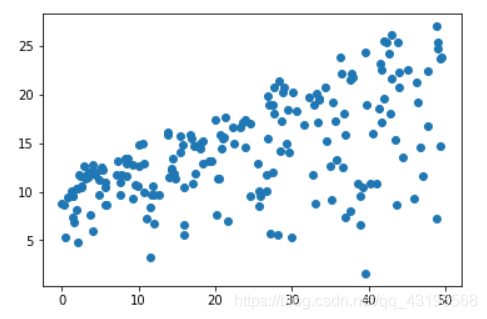
plt.scatter(data.radio, data.sales)
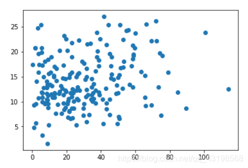
plt.scatter(data.newspaper, data.sales)

# 数据划分
x = data.iloc[:, 1:-1]
y = data.iloc[:, -1]

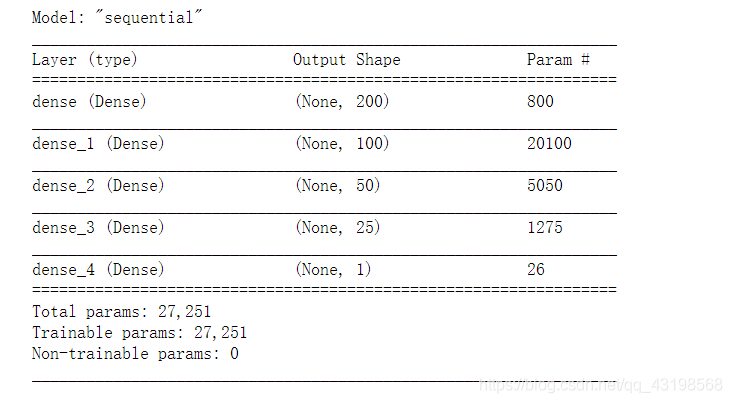
# 搭建神经网络
model = tf.keras.Sequential([tf.keras.layers.Dense(200, input_shape=(3,), activation='relu'),
                             tf.keras.layers.Dense(100, activation='relu'),
                             tf.keras.layers.Dense(50, activation='relu'),
                             tf.keras.layers.Dense(25, activation='relu'),
                            tf.keras.layers.Dense(1)])

print(model.summary())

# 设置优化模型、损失函数
model.compile(optimizer='adam', loss='mse')

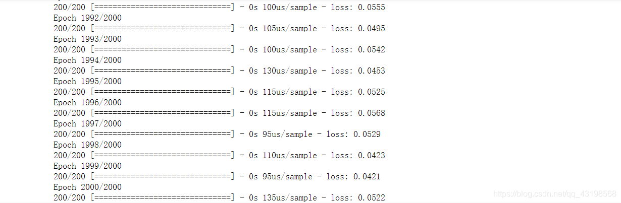
# 模型训练，迭代次数为2000
history = model.fit(x, y, epochs=2000)

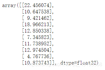
# 预测
test = data.iloc[:10, 1:-1]
model.predict(test)

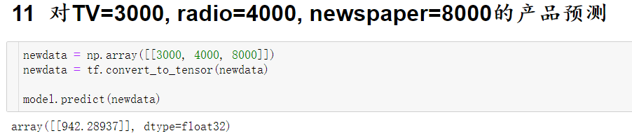
# 对TV=3000, radio=4000, newspaper=8000的产品预测
newdata = np.array([[3000, 4000, 8000]])
newdata = tf.convert_to_tensor(newdata)
model.predict(newdata)

结果