图像水平梯度和竖直梯度代码_三种梯度下降算法及代码实现

三种梯度算法：

1.批量梯度下降（BGD）

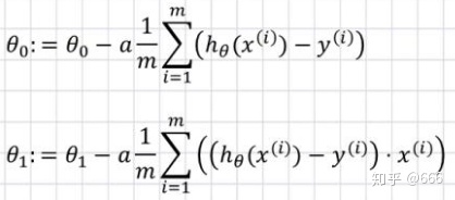
指在计算梯度下降的每一步中，我们都用到了所有的训练样本，在梯度下降中，在计算微积分时，我们需要进行求和运算。

2.随机梯度下降（SGD）

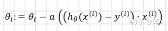
每次采用一个样本梯度下降

3.小批量梯度下降（MBGD）

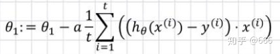
每次迭代使用一个以上又不是全部的样本

代码实现

1.导包和保存图片

import numpy as np
#导入操作系统
import os
#画图
%matplotlib inline
import matplotlib.pyplot as plt

# 随即种子
np.random.seed (42)

# 保存图片
PROJECT_ROOT_DIR="."
MODEL_ID ="linear_nodels"

def save_fig(fig_id,tight_layout=True):
    path=os.path.join(PROJECT_ROOT_DIR,"images",MODEL_ID,fig_id + ".png")
    print ("Saving figure",fig_id)
    plt.savefig(path,format = "png",dpi=300)
    
# 把讨厌的警告信息过滤掉
import warnings
warnings.filterwarnings(action="ignore",message="^internal gelsd")

2.创建原始数据并画图

X = 2*np.random.rand(100,1)
y = 4 + 3 * X + np.random.randn(100,1)

plt.plot(X,y,"b.")
plt.xlabel("$x_1$",fontsize=18)
plt.ylabel("$y$",rotation=0,fontsize=18)
save_fig("generated_data_plot")
plt.show()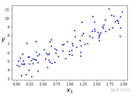

原始数据的散点图

3.导包做预测

# 添加新特征
X_b = np.c_[np.ones((100,1)),X]

# 创建测试数据
X_new=np.array([[0],[2]])
X_new_b=np.c_[np.ones((2,1)),X_new]

# 从sklearn 包里导入线性回归方程
from sklearn.linear_model import LinearRegression 
lin_reg=LinearRegression() #创建线性回归对象
lin_reg.fit(X,y)  #拟合训练数据
lin_reg.intercept_,lin_reg.coef_  #输出截距,斜率

输出的截距和斜率

# 对测试集进行预测
lin_reg.predict(X_new)

预测出X_new对应的y值

4.用批量梯度下降求解线性回归

#alpha（学习率）
eta=0.1
#运行次数
n_iterations=1000
m=100
theta = np.random.randn(2,1)

for iteration in range(n_iterations):
    gradients = 2/m * X_b.T.dot(X_b.dot(theta)-y)
    theta=theta - eta*gradients

定义函数

#用于只保存eta=0.1时的图像
theta_path_bgd=[]

def plot_gradient_descent(theta, eta, theta_path=None):
    m=len(X_b)
#     对数据画散点图
    plt.plot(X,y,"b.")
    
#     循环次数
    n_iterations = 1000
    for iteration in range(n_iterations):
        if iteration < 10:
            y_predict=X_new_b.dot(theta)
            style = "r-"
            plt.plot(X_new, y_predict, style)
#             梯度
        gradients = 2/m * X_b.T.dot(X_b.dot(theta) - y)
#     更新theta
        theta=theta-eta * gradients
    
        if theta_path is not None:
            theta_path.append(theta)
    plt.xlabel("$x_1$",fontsize=18)
    plt.axis([0,2,0,15])
    plt.title(r"$eta = {}$".format(eta),fontsize=16)
      

画不同

值时的图像

np.random.seed(42)
theta = np.random.randn(2,1) 

plt.figure(figsize=(10,4))
plt.subplot(131); plot_gradient_descent(theta, eta = 0.02)
plt.ylabel("$y$", rotation = 0, fontsize = 18)
plt.subplot(132); plot_gradient_descent(theta, eta=0.1,theta_path=theta_path_bgd)
plt.subplot(133); plot_gradient_descent(theta, eta = 0.5)

save_fig("gradient_descent_plot")
plt.show()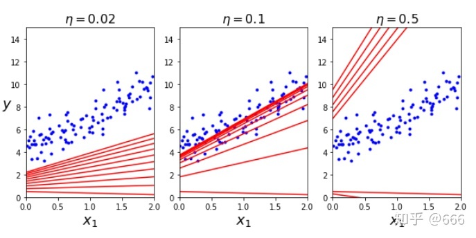

当alpha=0.02，0.1，0.5时，对应的图片

当

=0.1时拟合原数据

5.随机梯度下降

#存储每次 theta 更新的数据 
theta_path_sgd=[]
m = len(X_b)
np.random.seed(42)

#遍历的次数
n_epochs = 50

theta = np.random.randn(2,1) #随即初始化

for epoch in range (n_epochs):
    for i in range(m):
        if epoch == 0 and i < 20:
            y_predict = X_new_b.dot(theta)
            style = "r-"
            plt.plot(X_new, y_predict,style)
            random_index = np.random.randint(m)
            xi = X_b[random_index:random_index+1]
            yi = y[random_index:random_index+1]
            gradients = 2 * xi.T.dot(xi.dot(theta) - yi)
            eta = 0.1
            theta = theta - eta*gradients
            theta_path_sgd.append(theta)
            
plt.plot(X, y, "b.")
plt.xlabel("$x_1$",fontsize = 18)
plt.ylabel("$y$", rotation = 0, fontsize=18)
plt.axis([0,2,0,15])
save_fig("sgd_plot")
plt.show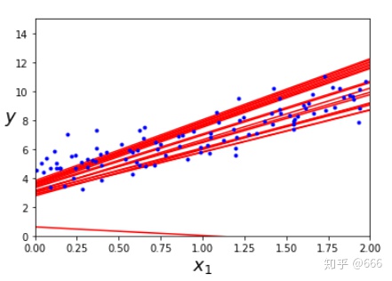

随机批量下降

调用写好的包

from sklearn.linear_model import SGDRegressor
sgd_reg = SGDRegressor(max_iter=5000,tol = -np.infty, penalty = None,eta0 = 0.1,random_state=42)
sgd_reg.fit(X, y.ravel())

sgd_reg.intercept_,sgd_reg.coef_

掉用包求出的截距和斜率

6.小批量梯度算法

定义函数：

theta_path_mgd = []

n_iterations = 50
minibatch_size = 20

np.random.seed(42)
theta = np.random.randn(2,1)

for epoch in range(n_iterations):
#     将数据打乱
    shuffled_indices = np.random.permutation(m)
    X_b_shuffled = X_b[shuffled_indices]
    y_shuffled = y[shuffled_indices]
    for i in range(0, m, minibatch_size):
        xi = X_b_shuffled[i:i+minibatch_size]
        yi = y_shuffled[i:i+minibatch_size]
        gradients = 2/minibatch_size * xi.T.dot(xi.dot(theta) - yi)
        eta = 0.1
        theta = theta - eta * gradients
        theta_path_mgd.append(theta)

7.总结三种方式并画图

theta_path_bgd = np.array(theta_path_bgd)
theta_path_sgd = np.array(theta_path_sgd)
theta_path_mgd = np.array(theta_path_mgd)

plt.figure(figsize=(7,4))
plt.plot(theta_path_sgd[:,0], theta_path_sgd[:,1], "r-s", linewidth=1, label="Stochastic")
plt.plot(theta_path_mgd[:,0], theta_path_mgd[:,1], "g-+", linewidth=2, label="Mini-batch")
plt.plot(theta_path_bgd[:,0], theta_path_bgd[:,1], "b-o", linewidth=3, label="Batch")
plt.legend(loc = "upper left",fontsize=16)
plt.xlabel(r"$theta_0$",fontsize=20)
plt.ylabel(r"$theta_1$",fontsize=20,rotation=0)
plt.axis([2.5,4.5,2.3,3.9])
save_fig("gradient_descent_plaths_plot")
plt.show()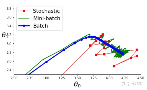

小批量梯度下降的算法比较好，它集中了批量梯度下降和随机梯度下降的优点。使多个样本相比SGD提高了梯度估计的精度