


参考《Python:数据科学手册》一书,仅作个人学习及记录使用,若有侵权,请联系后台删除。
1 理解Python中的数据类型
Numpy与Pandas是python中用来处理数字数组的主要工具,Numpy数组几乎是整个Python数据科学系统的核心。在现实生活中,我们看到的图片,视频,文字以及声音等都可以简单地看作是各种不同的数组,以便通过计算机的介入进行处理。数值数组的操作是数据科学的基石,本篇笔记是我的Numpy的入门笔记。
1.1 Python整型
标准的Python实现是用C语言写成。每一个python对象都是一个伪C语言结构体,该结构体不仅包含其值,还有其他信息。
struct_longobject{ long ob_refcnt; PyTypeObject *ob_type; size_t ob_size; long ob_digit[1];};
Python 3 里面的一个整型实际上包括 4 个部分。
ob_refcnt 是一个引用计数,它帮助 Python 默默地处理内存的分配和回收。ob_type 将变量的类型编码。ob_size 指定接下来的数据成员的大小。ob_digit 包含我们希望 Python 变量表示的实际整型值。
这意味着与C语言这样的编译型语言里的整型相比,在Python中存储一个整型会有一些额外的信息。
1.2 Python列表
Python中用来存储多元素的容器是列表,由于Python本身的特性,其列表中的每一项都包含了各自的类型的信息,引用计数以及其他信息。这使得为了表达该列表,Python背后所存储的信息比较冗余。而numpy式的数组是固定式的,虽然缺乏灵活性,却没有信息冗余,比较高效。
数组的创建
import numpy as npnp.array([1,4,2,5,3]) #整型数组array([1, 4, 2, 5, 3])np.array([3.14,4,2,3]) #Numpy要求数组必须包含同一类型的数据,如果类型不匹配,Numpy将向上转换。array([3.14, 4. , 2. , 3. ])np.array([1,2,3,4],dtype = 'float32') #通过dtype关键字可以设置明确的数据类型。array([1., 2., 3., 4.], dtype=float32)np.array([range(i,i+3) for i in [2,4,6]]) #嵌套列表构成的多维数组。array([[2, 3, 4],
[4, 5, 6],
[6, 7, 8]])np.zeros(10,dtype = int) #创建一个长度为10 的数组,数组的值都是0.array([0, 0, 0, 0, 0, 0, 0, 0, 0, 0])np.ones((3,5),dtype = float) #创建一个3*5的浮点型数组,数组的值都是1.array([[1., 1., 1., 1., 1.],
[1., 1., 1., 1., 1.],
[1., 1., 1., 1., 1.]])np.full((3,5),3.14) #创建一个3*5的浮点型数组,数组的值都是3.14.array([[3.14, 3.14, 3.14, 3.14, 3.14],
[3.14, 3.14, 3.14, 3.14, 3.14],
[3.14, 3.14, 3.14, 3.14, 3.14]])np.arange(0,20,2) #创建一个线性序列数组,从0开始,到20结束,步长为2,(和内置的range()函数类似)array([ 0, 2, 4, 6, 8, 10, 12, 14, 16, 18])np.linspace(0,1,5) #创建一个5个元素的数组,这5个数均匀地分配到0~1.array([0. , 0.25, 0.5 , 0.75, 1. ])np.random.random((3,3)) #创建一个3*3的,在0~1均匀分布的随机数组成的数组。array([[0.417411 , 0.22210781, 0.11986537],
[0.33761517, 0.9429097 , 0.32320293],
[0.51879062, 0.70301896, 0.3636296 ]])#创建一个3*3的,均值为0,标准差为1的
#正态分布的随机数数组。
np.random.normal(0,1,(3,3))array([[-0.0185508 , -1.67350462, -1.07253183],
[-0.99258618, 0.10234768, -0.43260928],
[-0.6591823 , 0.0039373 , 0.4777541 ]])#创建一个3*3的,[0,10]区间的随机整型数组。
np.random.randint(0,10,(3,3))array([[2, 1, 4],
[9, 5, 6],
[3, 6, 7]])#创建一个3*3的单位矩阵。
np.eye(3)array([[1., 0., 0.],
[0., 1., 0.],
[0., 0., 1.]])#创建一个由3个整型数组成的未初始化的数组
#数组的值是内存空间中的任意值。
np.empty(3)array([1., 1., 1.])2.1 Numpy数组的属性
一些有用的数组属性。ndim 数组的维度,shape 数组的每个维度的大小,size 数组的总大小,dtype 数组的数据类型,itemsize 每个数组元素字节大小,nbytes 数组总字节大小。
import numpy as np
np.random.seed(0)  #设置随机数种子
x1 = np.random.randint(10,size = 6) #一维数组
x2 = np.random.randint(10,size = (3,4))   #二维数组
x3 = np.random.randint(10,size = (3,4,5))   #三维数组
print(x1)
print(x2)
print(x3)
[5 0 3 3 7 9]
[[3 5 2 4]
[7 6 8 8]
[1 6 7 7]]
[[[8 1 5 9 8]
[9 4 3 0 3]
[5 0 2 3 8]
[1 3 3 3 7]]
[[0 1 9 9 0]
[4 7 3 2 7]
[2 0 0 4 5]
[5 6 8 4 1]]
[[4 9 8 1 1]
[7 9 9 3 6]
[7 2 0 3 5]
[9 4 4 6 4]]]
dtype: int32print("x3 ndim: ",x3.ndim) #ndim 数组的维度
print("x3 shape: ",x3.shape) # shape 数组的每个维度的大小
print("x3 size: ",x3.size) #size 数组的总大小
print("\ndtype:" ,x3.dtype) #dtype 数组的数据类型x3 ndim: 3
x3 shape: (3, 4, 5)
x3 size: 60
dtype: int32print("itemsize:",x3.itemsize,"bytes") #itemsize 每个数组元素字节大小
print("nbytes:",x3.nbytes,"bytes") # nbytes 数组总字节大小itemsize: 4 bytes
nbytes: 240 bytes2.2 数组索引:获取单个元素
和Python列表一样,在一维数组中,可以通过中括号指定索引获取第i个值。
x1array([5, 0, 3, 3, 7, 9])x1[0]5x1[4]7x1[-1]9x1[-2]7x2array([[3, 5, 2, 4], [7, 6, 8, 8], [1, 6, 7, 7]])x2[0,0] #在多维数组中,可以用逗号分隔的索引元组获取元素。3x2[0,0] = 12 #以索引方式修改元素。x2array([[12, 5, 2, 4],
[ 7, 6, 8, 8],
[ 1, 6, 7, 7]])x1[0] = 3.1415926 #和python列表不同,Numpy数组是固定类型的,这意味着当你将一个浮点数值插入一个整型数组时,浮点值会被截短成整型。
x1array([3, 0, 3, 3, 7, 9])数组切片:获取子数组
1 一维子数组
x = np.arange(10)
x
array([0, 1, 2, 3, 4, 5, 6, 7, 8, 9])x[:5]array([0, 1, 2, 3, 4])x[5:]array([5, 6, 7, 8, 9])x[4:7]array([4, 5, 6])x[::2]array([0, 2, 4, 6, 8])x[1::2]array([1, 3, 5, 7, 9])x[::-1]array([9, 8, 7, 6, 5, 4, 3, 2, 1, 0])x[5::-2]array([5, 3, 1])2.多维子数组
x2array([[12, 5, 2, 4],
[ 7, 6, 8, 8],
[ 1, 6, 7, 7]])x2[:2,:3]array([[12, 5, 2],
[ 7, 6, 8]])x2[:3,::2]array([[12, 2],
[ 7, 8],
[ 1, 7]])x2[::-1,::-1]array([[ 7, 7, 6, 1],
[ 8, 8, 6, 7],
[ 4, 2, 5, 12]])3.获取数组的行和列
x2[:,0]array([12, 7, 1])x2array([[12, 5, 2, 4],
[ 7, 6, 8, 8],
[ 1, 6, 7, 7]])x2[0,:]array([12, 5, 2, 4])x2[0]array([12, 5, 2, 4])4.非副本视图的子数组
x2array([[12, 5, 2, 4],
[ 7, 6, 8, 8],
[ 1, 6, 7, 7]])x2_sub = x2[:2,:2]
print(x2_sub)[[12 5]
[ 7 6]]x2_sub[0,0] = 99
print(x2_sub)
print(x2)[[99 5]
[ 7 6]]
[[99 5 2 4]
[ 7 6 8 8]
[ 1 6 7 7]]5.创建数组的副本
x2_sub_copy = x2[:2,:2].copy()
print(x2_sub_copy)
[[99 5]
[ 7 6]]x2_sub_copy[0,0] = 42print(x2_sub_copy)print(x2)[[42 5] [ 7 6]][[99 5 2 4] [ 7 6 8 8] [ 1 6 7 7]]2.4 数组的变形
grid = np.arange(1,10).reshape((3,3)) #数组变形最灵活的实现方式是通过reshape()函数来实现。print(grid)[[1 2 3] [4 5 6] [7 8 9]]x = np.array([1,2,3])xarray([1, 2, 3])x.reshape((1,3))array([[1, 2, 3]])x[np.newaxis,:]array([[1, 2, 3]])x.reshape((3,1))array([[1],
[2],
[3]])x[:,np.newaxis]array([[1],
[2],
[3]])2.5 数组的拼接与分裂
1 .数组的拼接:np.concatenate,np.vstack,np.hstack
import numpy as np
x = np.array([1,2,3])
y = np.array([3,2,1])
np.concatenate([x,y])
array([1, 2, 3, 3, 2, 1])z = ([99,99,99])
print(np.concatenate([x,y,z]))[ 1 2 3 3 2 1 99 99 99]grid = np.array([[1,2,3],
[4,5,6]])
np.concatenate([grid,grid])array([[1, 2, 3],
[4, 5, 6],
[1, 2, 3],
[4, 5, 6]])np.concatenate([grid,grid],axis = 1)array([[1, 2, 3, 1, 2, 3],
[4, 5, 6, 4, 5, 6]])x = np.array([1,2,3])
grid = np.array([[9,8,7],
[6,5,4]])
np.vstack([x,grid])array([[1, 2, 3], [9, 8, 7], [6, 5, 4]])grid = np.array([[9,8,7], [6,5,4]])y = np.array([[99], [99]])np.hstack([grid,y])array([[ 9, 8, 7, 99], [ 6, 5, 4, 99]])2 .数组的分裂分裂可以通过np.split,np.hsplit,np.vsplit函数来实现。
x = ([1,2,3,99,99,3,2,1])x1,x2,x3 = np.split(x,[3,5])print(x1,x2,x3)[1 2 3] [99 99] [3 2 1]grid = np.arange(16).reshape((4,4))gridarray([[ 0, 1, 2, 3], [ 4, 5, 6, 7], [ 8, 9, 10, 11], [12, 13, 14, 15]])upper, lower = np.vsplit(grid,[2])print(upper)print(lower)[[0 1 2 3]
[4 5 6 7]]
[[ 8 9 10 11]
[12 13 14 15]]left,right = np.hsplit(grid,[2])
print(left)
print(right)[[ 0 1]
[ 4 5]
[ 8 9]
[12 13]]
[[ 2 3]
[ 6 7]
[10 11]
[14 15]]3 numpy 数组的计算:通用函数
向量化的操作是Numpy计算变快的关键所在,通常该操作使用Numpy的通用函数来实现。
3.1:缓慢的循环
python的相对缓慢通常出现在很多小操作需要不断重复的时候,比如对数组的每个元素做循环操作时。这是因为之前提过的python的动态性和解释性。
import numpy as np
np.random.seed(0)
def compute_reciprocals(values):
    output = np.empty(len(values))
    for i in range(len(values)):
        output[i] = 1.0 / values[i]
    return output
values = np.random.randint(1,10,size = 5)
compute_reciprocals(values)
array([0.16666667, 1. , 0.25 , 0.25 , 0.125 ])big_array = np.random.randint(1,100,size = 1000000)%timeit compute_reciprocals(big_array)1.79 s ± 26 ms per loop (mean ± std. dev. of 7 runs, 1 loop each)3.2:通用函数介绍
Numpy为很多类型的操作提供了非常方便的,静态类型的,可编译程序的接口,也被称作向量操作。这种向量方法被用于将循环推送至Numpy之下的编译层,这样会取得更快的效率。
print(compute_reciprocals(values))print(1.0/values)[0.16666667 1. 0.25 0.25 0.125 ][0.16666667 1. 0.25 0.25 0.125 ]%timeit (1.0/big_array)3.49 ms ± 58.2 µs per loop (mean ± std. dev. of 7 runs, 100 loops each)np.arange(5)/np.arange(1,6)array([0. , 0.5 , 0.66666667, 0.75 , 0.8 ])x = np.arange(9).reshape((3,3))2**xarray([[ 1, 2, 4], [ 8, 16, 32], [ 64, 128, 256]], dtype=int32)3.3 探索NumPy的通用函数
1.数组的运算
x = np.arange(4)print("x = ",x)print("x + 5 = ",x+5)print("x - 5 = ",x-5)print("x * 2 = ",x*2)print("x / 2 = ",x/2)print("x //2 = ",x//2)print("x** 2 = ",x**2)print("x % 2 = ",x%2)print("-x = ",-x)x = [0 1 2 3]x + 5 = [5 6 7 8]x - 5 = [-5 -4 -3 -2]x * 2 = [0 2 4 6]x / 2 = [0. 0.5 1. 1.5]x //2 = [0 0 1 1]x** 2 = [0 1 4 9]x % 2 = [0 1 0 1]-x = [ 0 -1 -2 -3]2.绝对值
x = np.array([-2,-1,0,1,2])
abs(x)
array([2, 1, 0, 1, 2])np.absolute(x)array([2, 1, 0, 1, 2])x= np.array([3 - 4j,4-3j,2+0j,0+1j])
np.abs(x)array([5., 5., 2., 1.])3.三角函数
theta = np.linspace(0,np.pi,3)
print("theta        = ",theta)
print("sin(theta)   = ",np.sin(theta))
print("cos(theta)   = ",np.cos(theta))
print("tan(theta)   = ",np.tan(theta))
x = [-1,0,1]
print("x = ",x)
print("arcsin(x) = ",np.arcsin(x))
print("arccos(x) = ",np.arccos(x))
print("arctan(x) = ",np.arctan(x))4.指数和对数
x = [1,2,3]
print("x        = ",x)
print("e^x      = ",np.exp(x))
print("2^x      = ",np.exp2(x))
print("3^x      = ",np.power(3,x))
x = [1,2,4,10]
print("x = ",x)
print("ln(x) = ",np.log(x))
print("log2(x) = ",np.log2(x))
print("log10(x) = ",np.log10(x))x= [0,0.001,0.01,0.1]
print("exp(x) - 1 = ",np.expm1(x))
print("log(1+x) = ",np.log1p(x))5.专用的通用函数
from scipy import special
x= [1,5,10]
print("gamma(x)     = ",special.gamma(x))
print("ln|gamma(x)| = ",special.gammaln(x))
print("beta(x,2)    = ",special.beta(x,2))
x = np.array([0,0.3,0.7,1.0])
print("erf(x) = ",special.erf(x))
print("erfc(x) = ",special.erfc(x))
print("erfinv(x)= ",special.erfinv(x))3.4 高级的通用函数特性
1 指定输出
x = np.arange(5)
y = np.empty(5)
np.multiply(x,10,out=y)
print(y)
[ 0. 10. 20. 30. 40.]y = np.zeros(10)
np.power(2,x,out = y[::2])
print(y)[ 2. 0. 4. 0. 8. 0. 16. 0. 32. 0.]2 聚合
x= np.arange(1,6)
print(x)
np.add.reduce(x)
[1 2 3 4 5]15np.multiply.reduce(x)120np.add.accumulate(x)array([ 1, 3, 6, 10, 15], dtype=int32)np.multiply.accumulate(x)array([ 1, 2, 6, 24, 120], dtype=int32)3 外积
x = np.arange(1,6)np.multiply.outer(x,x)array([[ 1, 2, 3, 4, 5], [ 2, 4, 6, 8, 10], [ 3, 6, 9, 12, 15], [ 4, 8, 12, 16, 20], [ 5, 10, 15, 20, 25]])4 聚合 :最小值,最大值和其他值
4.1 数组值求和
import numpy as npL= np.random.random(100)sum(L)np.sum(L)big_array = np.random.rand(1000000)%timeit sum(big_array)%timeit np.sum(big_array)4.2 最小值和最大值
min(big_array)max(big_array)np.min(big_array)np.max(big_array)%timeit min(big_array)%timeit np.min(big_array)print(big_array.min(),big_array.max(),big_array.sum())1.多维度聚合
M = np.random.random((3,4))print(M)M.sum()M.min(axis=0)M.max(axis = 1)4.3 示例:美国总统的身高是多少
import numpy as np
import pandas as pd
data = pd.read_csv("data/president_heights.csv")
heights = np.array(data["height(cm)"])
print(heights)
print("Mean height : ",heights.mean())
print("Standard deviation : ",heights.std())
print("Minimum height : ",heights.min())
print("Maximum height : ",heights.max())print("25th percentile: ",np.percentile(heights,25))
print("Median: ",np.median(heights))
print("75th percentile: ",np.percentile(heights,75))%matplotlib inline
import matplotlib.pyplot as plt
import seaborn;seaborn.set()plt.hist(heights)
plt.title("Height Distribution of US Presidents")
plt.xlabel("height(cm)")
plt.ylabel("number");5 数组的计算:广播
5.1 广播的介绍
import numpy as np
a = np.array([0,1,2])
b = np.array([5,5,5])
a+barray([5, 6, 7])a + 5array([5, 6, 7])M= np.ones((3,3))
Marray([[1., 1., 1.],
[1., 1., 1.],
[1., 1., 1.]])M+aarray([[1., 2., 3.],
[1., 2., 3.],
[1., 2., 3.]])a = np.arange(3)
b = np.arange(3)[:,np.newaxis]
print(a)
print(b)[0 1 2]
[[0]
[1]
[2]]a+barray([[0, 1, 2],
[1, 2, 3],
[2, 3, 4]])5.2 广播的规则
1:广播示例1
M = np.ones((2,3))
a = np.arange(3)M+aarray([[1., 2., 3.],
[1., 2., 3.]])2:广播示例2
a = np.arange(3).reshape((3,1))
b = np.arange(3)
a+barray([[0, 1, 2],
[1, 2, 3],
[2, 3, 4]])3:广播示例3
M = np.ones((3,2))
a = np.arange(3)[:,np.newaxis]
M+aarray([[1., 1.],
[2., 2.],
[3., 3.]])np.logaddexp(M,a)array([[1.31326169, 1.31326169],
[1.69314718, 1.69314718],
[2.31326169, 2.31326169]])5.3 广播的实际应用
1:数组的归一化
X = np.random.random((10,3))
Xmean = X.mean(0)
Xmeanarray([0.52810714, 0.50478518, 0.69315893])X_centered = X - XmeanX_centered.mean(0)array([-2.22044605e-17, 0.00000000e+00, 4.44089210e-17])2:画一个二维函数
x = np.linspace(0,5,50)
y = np.linspace(0,5,50)[:,np.newaxis]
z = np.sin(x)**10 + np.cos(10 + y*x)*np.cos(x)%matplotlib inline
import matplotlib.pyplot as plt
plt.imshow(z,origin = "lower",extent = [0,5,0,5],
cmap = "viridis")
plt.colorbar();
6 比较,掩码和布尔逻辑
掩码用于基于某些准则抽取,修改,计数或对一个数组中的值进行各种各样的操作。6.1 示例:统计下雨天数
import numpy as np
import pandas as pd
rainfall = pd.read_csv("data/Seattle2014.csv")['PRCP'].values
inches = rainfall / 254
inches.shape(365,)%matplotlib inline
import matplotlib.pyplot as plt
import seaborn;seaborn.set()
plt.hist(inches,40);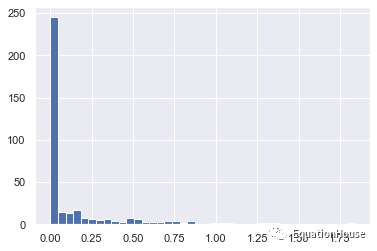
6.2 和通用函数类似的比较操作
x = np.array([1,2,3,4,5])
x<3array([ True, True, False, False, False])x>3array([False, False, False, True, True])x<=3array([ True, True, True, False, False])x>=3array([False, False, True, True, True])x != 3array([ True, True, False, True, True])x == 3array([False, False, True, False, False])(2**x) == (x ** 2)array([False, True, False, True, False])rng = np.random.RandomState(0)
x = rng.randint(10,size = (3,4))
xarray([[5, 0, 3, 3],
[7, 9, 3, 5],
[2, 4, 7, 6]])x<6array([[ True, True, True, True],
[False, False, True, True],
[ True, True, False, False]])6.3 操作布尔数组
print(x)[[5 0 3 3]
[7 9 3 5]
[2 4 7 6]]1.统计记录的个数
np.count_nonzero(x<6)8np.sum(x<6,axis = 1)array([4, 2, 2])np.any(x>8)Truenp.all(x<10)Truenp.all(x == 6)Falsenp.all(x<8,axis = 0)array([ True, False, True, True])np.all(x<8,axis = 1)array([ True, False, True])2 布尔运算符
import numpy as np
import pandas as pd
rainfall = pd.read_csv("data/Seattle2014.csv")['PRCP'].values
inches = rainfall / 254
np.sum((inches > 0.5) & (inches < 1))29np.sum(~((inches <= 0.5)|(inches >= 1)))29print("Number days without rain: ",np.sum(inches == 0))
print("Number days with rain: ",np.sum(inches != 0))
print("Days with more than 0.5 inches : ",np.sum(inches > 0.5))
print("Rainy days with < 0.2 inches : ",np.sum((inches > 0)&(inches < 0.2)))Number days without rain: 215
Number days with rain: 150
Days with more than 0.5 inches : 37
Rainy days with < 0.2 inches : 752.6.4 将布尔数组作为掩码
rng = np.random.RandomState(0)
x = rng.randint(10,size = (3,4))
xarray([[5, 0, 3, 3],
[7, 9, 3, 5],
[2, 4, 7, 6]])x<5array([[False, True, True, True],
[False, False, True, False],
[ True, True, False, False]])x[x<5]array([0, 3, 3, 3, 2, 4])rainy = (inches > 0)summer = (np.arange(365)-172 < 90) & (np.arange(365)-172 > 0)print("Median precip on rainy days in 2014 (inches): ",
np.median(inches[rainy]))
print("Median precip on summer days in 2014 (inches): ",
np.median(inches[summer]))
print("Maximum precip on summer days in 2014 (inches): ",
np.max(inches[summer]))
print("Median precip on non-summer rainy days(inches): ",
np.median(inches[rainy & ~summer]))Median precip on rainy days in 2014 (inches): 0.19488188976377951
Median precip on summer days in 2014 (inches): 0.0
Maximum precip on summer days in 2014 (inches): 0.8503937007874016
Median precip on non-summer rainy days(inches): 0.200787401574803157 花哨的索引
7.1 探索花哨的索引
import numpy as np
rand = np.random.RandomState(42)
x = rand.randint(100,size = 10)
print(x)[51 92 14 71 60 20 82 86 74 74][x[3],x[7],x[2]][71, 86, 14]ind = [3,7,4]
x[ind]array([71, 86, 60])ind = np.array([[3,7],
[4,5]])
x[ind]array([[71, 86],
[60, 20]])X = np.arange(12).reshape((3,4))
Xarray([[ 0, 1, 2, 3],
[ 4, 5, 6, 7],
[ 8, 9, 10, 11]])row = np.array([0,1,2])
col = np.array([2,1,3])
X[row,col]array([ 2, 5, 11])X[row[:,np.newaxis],col]array([[ 2, 1, 3],
[ 6, 5, 7],
[10, 9, 11]])row[:,np.newaxis]*colarray([[0, 0, 0],
[2, 1, 3],
[4, 2, 6]])7.2 组合索引
X = np.arange(12).reshape((3,4))
Xarray([[ 0, 1, 2, 3],
[ 4, 5, 6, 7],
[ 8, 9, 10, 11]])X[2,[2,0,1]]array([10, 8, 9])X[1:,[2,0,1]]array([[ 6, 4, 5],
[10, 8, 9]])mask = np.array([1,0,1,0],dtype = bool)
X[row[:,np.newaxis],mask]array([[ 0, 2],
[ 4, 6],
[ 8, 10]])7.3 示例:选择随机点
mean = [0,0]
cov = [[1,2],
[2,5]]
X= rand.multivariate_normal(mean,cov,100)
X.shape(100, 2)%matplotlib inline
import matplotlib.pyplot as plt
import seaborn ; seaborn.set()
plt.scatter(X[:,0],X[:,1])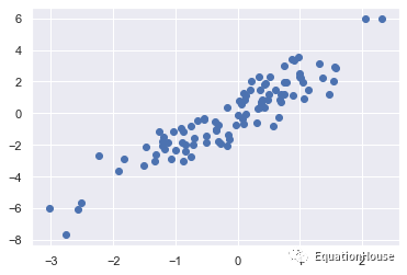
indices = np.random.choice(X.shape[0],20,replace = False)indicesarray([60, 80, 95, 33, 12, 25, 20, 50, 8, 72, 70, 51, 59, 92, 45, 21, 49,
42, 73, 2])selection = X[indices]
selection.shape(20, 2)plt.scatter(X[:,0],X[:,1],alpha = 0.3)
plt.scatter(selection[:,0],selection[:,1],
facecolor = 'none',edgecolor = 'b',s = 200)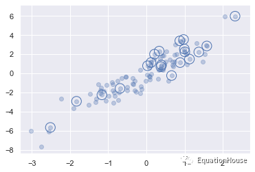
7.4 用花哨的索引修改值
x = np.arange(10)
i = np.array([2,1,8,4])
x[i] = 99
print(x)[ 0 99 99 3 99 5 6 7 99 9]x[i] -= 10print(x)[ 0 89 89 3 89 5 6 7 89 9]x = np.zeros(10)x[[0,0]] = [4,6]print(x)[6. 0. 0. 0. 0. 0. 0. 0. 0. 0.]i = [2,3,3,4,4,4]x[i] += 1xarray([6., 0., 1., 1., 1., 0., 0., 0., 0., 0.])x = np.zeros(10)np.add.at(x,i,1)print(x)[0. 0. 1. 2. 3. 0. 0. 0. 0. 0.]7.5 示例:数据区间划分
import sysnp.random.seed(42)x = np.random.randn(100)bins = np.linspace(-5,5,20)counts = np.zeros_like(bins)i = np.searchsorted(bins,x)np.add.at(counts,i,1)plt.plot(bins,counts,linestyle = "steps");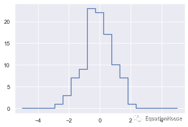
plt.hist(x,bins,histtype = "step");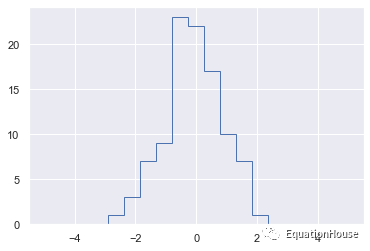
print("Numpy routine: ")%timeit counts,edges = np.histogram(x,bins)print("Custom routine: ")%timeit np.add.at(counts,np.searchsorted(bins,x),1)Numpy routine:21.3 µs ± 107 ns per loop (mean ± std. dev. of 7 runs, 10000 loops each)Custom routine:11.5 µs ± 24.7 ns per loop (mean ± std. dev. of 7 runs, 100000 loops each)x = np.random.randn(1000000)print("Numpy routine: ")%timeit counts,edges = np.histogram(x,bins)print("Custom routine: ")%timeit np.add.at(counts,np.searchsorted(bins,x),1)Numpy routine:53.1 ms ± 76.2 µs per loop (mean ± std. dev. of 7 runs, 10 loops each)Custom routine:88.5 ms ± 271 µs per loop (mean ± std. dev. of 7 runs, 10 loops each)8 数组的排序
import numpy as np
def selection_sort(x):
for i in range(len(x)):
swap = i + np.argmin(x[i:])
(x[i],x[swap]) = (x[swap],x[i])
return x
x = np.array([2,1,4,3,5])
selection_sort(x)array([1, 2, 3, 4, 5])def bogosort(x):
while np.any(x[:-1] > x[1:]):
np.random.shuffle(x)
return x
x = np.array([2,1,4,3,5])
bogosort(x)array([1, 2, 3, 4, 5])8.1 Numpy中的快速排序:np.sort 和 np.argsort
x = np.array([2,1,4,3,5])
np.sort(x)array([1, 2, 3, 4, 5])x.sort()
print(x)[1 2 3 4 5]x = np.array([2,1,4,3,5])
i = np.argsort(x)
print(i)[1 0 3 2 4]x[i]array([1, 2, 3, 4, 5])rand = np.random.RandomState(42)
X = rand.randint(0,10,(4,6))
print(X)[[6 3 7 4 6 9]
[2 6 7 4 3 7]
[7 2 5 4 1 7]
[5 1 4 0 9 5]]np.sort(X,axis = 0)array([[2, 1, 4, 0, 1, 5],
[5, 2, 5, 4, 3, 7],
[6, 3, 7, 4, 6, 7],
[7, 6, 7, 4, 9, 9]])np.sort(X,axis = 1)array([[3, 4, 6, 6, 7, 9],
[2, 3, 4, 6, 7, 7],
[1, 2, 4, 5, 7, 7],
[0, 1, 4, 5, 5, 9]])8.2 部分排序,分隔
x = np.array([7,2,3,1,6,5,4])
np.partition(x,3)array([2, 1, 3, 4, 6, 5, 7])np.partition(X,2,axis = 1)array([[3, 4, 6, 7, 6, 9],
[2, 3, 4, 7, 6, 7],
[1, 2, 4, 5, 7, 7],
[0, 1, 4, 5, 9, 5]])X = rand.rand(10,2)
%matplotlib inline
import matplotlib.pyplot as plt
import seaborn;seaborn.set()
plt.scatter(X[:,0],X[:,1],s=100);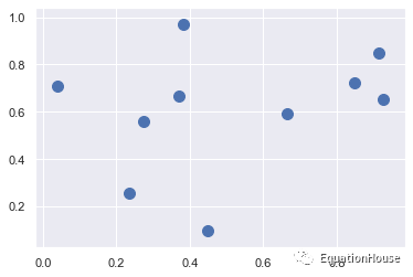
dist_sq = np.sum((X[:,np.newaxis,:] - X[np.newaxis,:,:])**2,axis = -1)
print(dist_sq)
[[0. 0.03971432 0.53615183 0.30887652 0.07137053 0.43262538
0.39806216 0.01098053 0.632568 0.78831133]
[0.03971432 0. 0.78616274 0.32892236 0.12896638 0.49330719
0.29786335 0.02082527 0.81380738 0.78422146]
[0.53615183 0.78616274 0. 0.33500633 0.29276457 0.24753085
0.77233057 0.5518468 0.07137869 0.54583095]
[0.30887652 0.32892236 0.33500633 0. 0.09309942 0.02081182
0.09187737 0.23137254 0.18856152 0.11090307]
[0.07137053 0.12896638 0.29276457 0.09309942 0. 0.15394115
0.22480149 0.05049831 0.29722499 0.40548423]
[0.43262538 0.49330719 0.24753085 0.02081182 0.15394115 0.
0.18019287 0.35545228 0.09463239 0.07721714]
[0.39806216 0.29786335 0.77233057 0.09187737 0.22480149 0.18019287
0. 0.27963512 0.53373795 0.18544834]
[0.01098053 0.02082527 0.5518468 0.23137254 0.05049831 0.35545228
0.27963512 0. 0.59252219 0.65376276]
[0.632568 0.81380738 0.07137869 0.18856152 0.29722499 0.09463239
0.53373795 0.59252219 0. 0.24489654]
[0.78831133 0.78422146 0.54583095 0.11090307 0.40548423 0.07721714
0.18544834 0.65376276 0.24489654 0. ]]differences = X[:,np.newaxis,:] - X[np.newaxis,:,:]
differences.shape(10, 10, 2)sq_differences = differences**2
sq_differences.shape(10, 10, 2)dist_sq = sq_differences.sum(-1)
dist_sq.shape(10, 10)dist_sq.diagonal()array([0., 0., 0., 0., 0., 0., 0., 0., 0., 0.])nearest = np.argsort(dist_sq,axis = 1)
print(nearest)[[0 7 1 4 3 6 5 2 8 9]
[1 7 0 4 6 3 5 9 2 8]
[2 8 5 4 3 0 9 7 6 1]
[3 5 6 4 9 8 7 0 1 2]
[4 7 0 3 1 5 6 2 8 9]
[5 3 9 8 4 6 2 7 0 1]
[6 3 5 9 4 7 1 0 8 2]
[7 0 1 4 3 6 5 2 8 9]
[8 2 5 3 9 4 6 7 0 1]
[9 5 3 6 8 4 2 7 1 0]]K=2
nearest_partition = np.argpartition(dist_sq,K+1,axis = 1)plt.scatter(X[:,0],X[:,1],s = 100)
plt.scatter(X[:,0],X[:,1],s = 100)
K = 2
for i in range(X.shape[0]):
    for j in nearest_partition[i,:K+1]:
        plt.plot(*zip(X[j],X[i]),color = "black")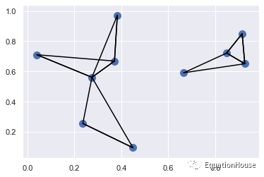
9 结构化数据:NumPy的结构化数组
name = ['Alice','Bob','Cathy','Doug']age = [25,45,37,19]weight = [55.0,85.5,68.0,61.5]import numpy as npx = np.zeros(4,dtype = int)data = np.zeros(4,dtype = {'names':('name','age','weight'), 'formats':('U10','i4','f8')})print(data.dtype)[('name', 'data['name'] = namedata['age']=agedata['weight'] = weightprint(data)[('Alice', 25, 55. ) ('Bob', 45, 85.5) ('Cathy', 37, 68. ) ('Doug', 19, 61.5)]data['name']array(['Alice', 'Bob', 'Cathy', 'Doug'], dtype='data[0]('Alice', 25, 55.)data[-1]['name']'Doug'data[data['age']<30]['name']array(['Alice', 'Doug'], dtype='9.1 生成结构化数组
np.dtype({'names':('name','age','weight'), 'formats':('U10','i4','f8')})dtype([('name', 'np.dtype({'names':('name','age','weight'), 'formats':((np.str_,10),int,np.float32)})dtype([('name', 'np.dtype([('name','S10'),('age','i4'),('weight','f8')])dtype([('name', 'S10'), ('age', 'np.dtype('S10,i4,f8')dtype([('f0', 'S10'), ('f1', '9.2 更高级的复合类型
tp = np.dtype([('id','i8'),('mat','f8',(3,3))])X=np.zeros(1,dtype = tp)print(X[0])print(X['mat'][0])(0, [[0., 0., 0.], [0., 0., 0.], [0., 0., 0.]])[[0. 0. 0.] [0. 0. 0.] [0. 0. 0.]]9.3 记录数组:结构化数组的扭转
data['age']array([25, 45, 37, 19])data_rec = data.view(np.recarray)data_rec.agearray([25, 45, 37, 19])%timeit data['age']%timeit data_rec['age']%timeit data_rec.age128 ns ± 12.2 ns per loop (mean ± std. dev. of 7 runs, 10000000 loops each)2.07 µs ± 32.3 ns per loop (mean ± std. dev. of 7 runs, 100000 loops each)2.76 µs ± 5.66 ns per loop (mean ± std. dev. of 7 runs, 100000 loops each)


 5820
5820


 被折叠的 条评论
为什么被折叠?
被折叠的 条评论
为什么被折叠?
 到【灌水乐园】发言


