CMU-15445 学习笔记总结（1）

最新推荐文章于 2024-03-18 03:13:28 发布

LittleSnailoo

最新推荐文章于 2024-03-18 03:13:28 发布

阅读量1.3k

点赞数

分类专栏：数据库文章标签：数据库开发分布式 database

本文链接：https://blog.csdn.net/weixin_40448099/article/details/129582393

版权

数据库专栏收录该内容

4 篇文章 0 订阅

订阅专栏

1.Hash Tables

2.B+ Trees

3.Index Concurrency Control

4.Sorting & Aggregations

5.Joins

6.Query Execution I

7.Query Executin II 并发

8.Query Optimization 查询优化

9.Query OptimizationII : Statistics and plan enumeration

1.Hash Tables

使用hash table的地方：
1. internal meta-data
2. core data storage
3. temporary data structures
4. table indexs【hash表不适于范围查询】
设计hash table时的考虑：
1. data organization：我们如何在内存/页面中布局数据结构，以及存储哪些信息以支持有效的访问。
2. concurrenty：如何使多个线程同时访问数据结构而不引起问题
hash table定义：
1. 哈希表实现了将键映射到值的无序关联数组。它使用哈希函数计算给定键在数组中的偏移量，从中可以找到所需的值。
2. Space Complexity: O(n)
3. Time Complexity: → Average: O(1) → Worst: O(n)
hash table 分类
1. static hash table：分配一个大数组，每个元素都有一个插槽。要查找一个条目，将键值乘以元素的数量，以查找数组中的偏移量
hash table 设计：
1. hash function：→ How to map a large key space into a smaller domain. → Trade-off between being fast vs. collision rate.
2. Hashing Scheme：→ How to handle key collisions after hashing. → Trade-off between allocating a large hash table vs. additional instructions to find/insert keys（在分配大哈希表与查找/插入键的额外指令之间进行权衡）
hash function
1. CRC-64 (1975)→ Used in networking for error detection.（redis）
2. MurmurHash (2008)→ Designed as a fast, general-purpose hash function.
3. Google CityHash (2011)→ Designed to be faster for short keys (
4. Facebook XXHash (2012)→ From the creator of zstd compression.
5. Google FarmHash (2014)→ Newer version of CityHash with better collision rates.
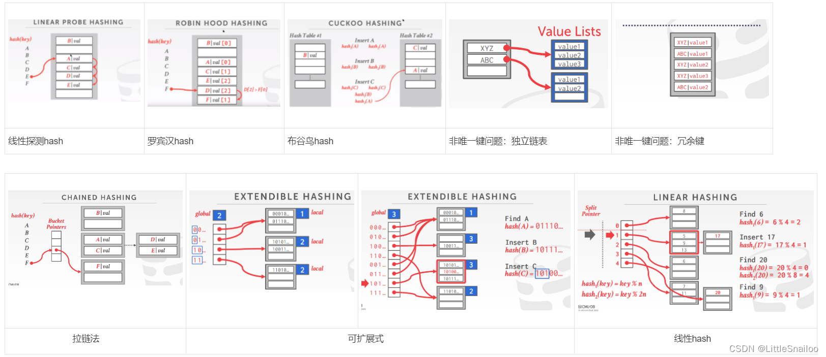
static hashing schemes
1. Linear Probe Hashing 线性探测哈希/开放地址哈希
  1. delete时会有问题：Approach #1: Tombstone Approach #2: Movement
  2. 非唯一键问题：Choice #1: Separate Linked List（独立链表）：将每个键的值存储在单独的存储区域；Choice #2: Redundant Keys（冗余键）：将重复的键项存储在哈希表中
2. Robin Hood Hashing 罗宾汉哈希
3. Cuckoo Hashing 布谷鸟哈希
4. 以上三种hash存储方式，都需要知道存储元素的总数目（槽数一定）属于静态hash表，不能动态伸缩
Dynamic hash tables
1. Chained Hashing 拉链式（1. java hash map实现类似，桶容量为1，桶个数多时转换为红黑树；2. go map实现类似，第一个桶容量为8（结构体中有一个数组8byte）之后有溢出桶）
2. Extendible Hashing 可扩展式
3. Linear Hashing 线性hash

2.B+ Trees

table index：表索引是表属性子集的副本，这些属性是为了使用这些属性进行高效访问而组织和/或排序的。DBMS确保表和索引的内容在逻辑上同步。DBMS的工作是找出用于执行每个查询的最佳索引。对于每个数据库要创建的索引数量，需要进行权衡。1. Storage Overhead 存储开销 2. Maintenance Overhead 维护费用
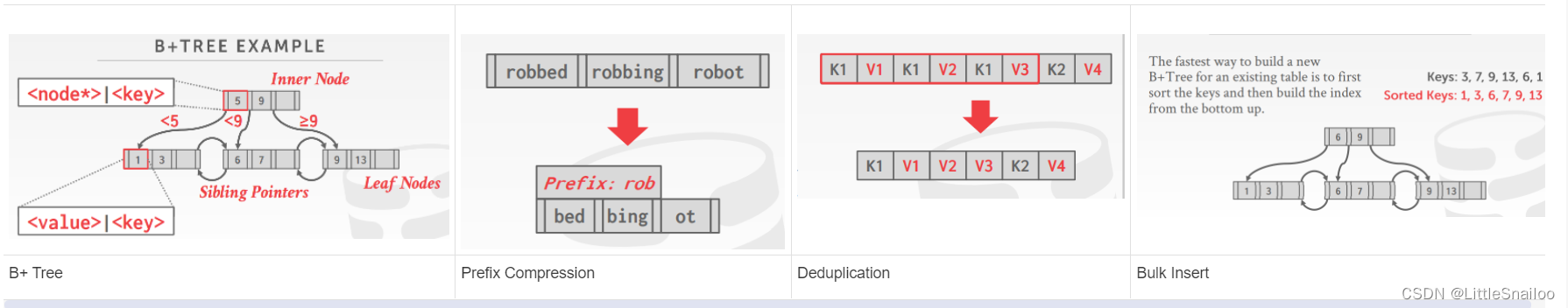
B+Tree Overview
1. B Tree Family： → B-Tree (1971) → B+Tree (1973) → B*Tree (1977?) → Blink-Tree (1981)
2. B+树是一种自平衡的树数据结构，它保持数据排序，并允许在O(log n)内进行搜索、顺序访问、插入和删除。1. 二叉搜索树的泛化，因为一个节点可以有两个以上的子节点。2. 针对读写大数据块的系统进行优化。
3. B+树是M-way搜索树，具有以下属性:
  1. →它是完美平衡的(即，每个叶节点在树中处于相同的深度)
  2. →除根节点外的每个节点至少是半满的M/2-1≤#keys≤M-1
  3. →每个有k个键的内部节点都有k+1个非空子节点
  4. node节点是一组kv，叶子节点v是数据【Record IDs，or Tuple Data】，内部节点v是索引
4. b tree：More space-efficient, since each key only appears once in the tree； b+ tree：A B+Tree only stores values in leaf nodes. Inner nodes only guide the search process.
Use in a DBMS
1. b+ tree支持的搜索：Example: Index on<a, b, c>
  1. Example: Index on → Supported: (b=3) 【跳跃搜索】
  2. Example: Index on → Supported: (a=5 AND b=3)
2. b+ tree duplicate keys ： Approach #1: Append Record ID； Approach #2: Overflow Leaf Nodes
3. clustered indexes 聚簇索引：The table is stored in the sort order specified by the primary key. 聚簇索引存储的数据，index与实际存储在磁盘上的数据一致
Design Choices
1. Node Size:
  1. The slower the storage device, the larger the optimal node size for a B+Tree. → HDD: ~1MB → SSD: ~10KB → In-Memory: ~512B 【16k】
  2. Optimal sizes can vary depending on the workload → Leaf Node Scans vs. Root-to-Leaf Traversals 【AP(大节点) vs. TP(小节点)】
2. Merge Threshold 节点合并的阈值：
  1. 有些dbms在节点满一半时并不总是合并节点。延迟合并操作可能会减少重组的数量。让更小的节点存在，然后周期性地重建整个树可能会更好。
3. Variable-Length Keys 变长的键：
  1. Approach #1: Pointers→ Store the keys as pointers to the tuple’s attribute.
  2. Approach #2: Variable-Length Nodes→ The size of each node in the index can vary.→ Requires careful memory management.
  3. Approach #3: Padding→ Always pad the key to be max length of the key type.
  4. Approach #4: Key Map / Indirection→ Embed an array of pointers that map to the key + value list within the node.
4. Intra-Node Search 内部节点搜索：
  1. Approach #1: Linear→ Scan node keys from beginning to end.【已加载到内存中的数据，直接找】
  2. Approach #2: Binary→ Jump to middle key, pivot left/right depending on comparison.【二分】
  3. Approach #3: Interpolation→ Approximate location of desired key based on known distribution of keys【找规律推断目标数据位置】
Optimizations b+ 树优化
1. Prefix Compression： Sorted keys in the same leaf node are likely to have the same prefix.Instead of storing the entire key each time, extract common prefix and store only unique suffix for each key.
2. Deduplication：
3. Bulk Insert：
4. Many more…

3.Index Concurrency Control

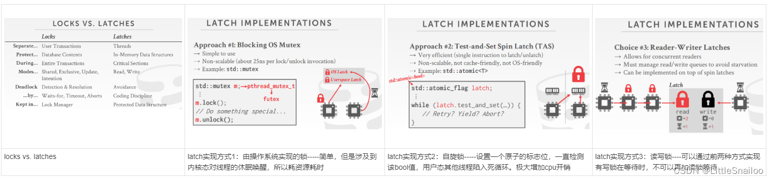
locks vs. latches:
1. Locks: 逻辑的宏观的锁
  1. 保护数据库的逻辑内容不受其他txns的影响。
  2. 保持txn时间。
  3. 需要能够回滚更改。
2. Latches：物理的微观的锁
  1. 保护DBMS内部数据结构的关键部分不受其他线程的影响。
  2. 操作持续时间
  3. 不需要能够回滚更改。
Latch Modes：读共享写独占
1. Read Mode
2. Write Mode
Latch 实现方式
1. Blocking OS Mutex
2. Test-and-Set Spin Latch (TAS)
3. Reader-Writer Latches
Hash Table Latching
1. hash表实现latch比较容易，因为hash表所有线程都朝一个方向运动，一次只访问一个页面/槽，不会出现死锁。
2. Approach #1: Page Latches：hash存储按页分段，给整个页加锁
3. Approach #2: Slot Latches：给整个槽加锁，粒度更小 【go map不支持并发，sync.Map支持并发】
Hash insert 可以 no latch：【Compare And Sarp： __sync_bool_compare_and_swap(&M, 20, 30) 硬件层面提供的原子操作】
B+Tree Latching
1. b+树需要考虑加锁的两种情况：（1）同时尝试修改节点内容的线程。（2）一个线程遍历树，另一个线程拆分/合并节点。
2. Latch Crabbing/Coupling: 插入删除修改都加写锁，查找加读锁【悲观】
  1. 基本思想: →为父母上锁
  2. →给孩子上锁
  3. →如果“安全”，为父母解锁
  4. 安全节点是指在更新时不会分裂或合并的节点。未满(插入时) 超过半满(删除时)
3. b+树加锁的改进：每次在根节点上执行写锁都会成为并发性较高的瓶颈。优化方式1：改为乐观加锁：增删改查在根节点都加读锁，叶子节点更改时判断若会引起上层节点变化，则返回从头开始加写锁
Leaf Node Scans
1. Leaf Node Scans：会出现死锁情况【T1: 1更改】Latch锁没有死锁检测或避免的机制，需要人为规范（例如：b+树不允许倒序遍历）

4.Sorting & Aggregations

Sorting：

Query Plan：操作符被排列在树中，数据从树的叶子流向根，根节点的输出是查询的结果
Disk-Oriented DBMS:需要依赖缓存池去执行算子，最大化利用连续读写io（sequential I/O）
如果数据都可以加载到内存中，则可以直接使用常见的排序算法进行Sort算子的执行，如冒泡，快排等；如果数据量很大，不可以一次性加载到内存，最常使用的排序方式是：External Merge Sort【外部归并排序】
Sorted Run：一组key/value值进行排序，有两种方式：1.key排序时，tuple也都排序好（早物化）2. key排序时，只排好Record ID，之后再进行回表（晚物化）
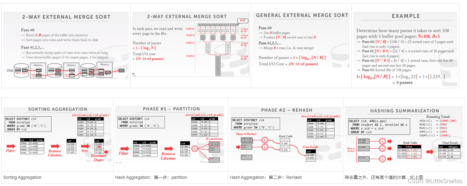
2-way External Merge Sort 内存中仅需要3个页（16k*3）就够了。内存多时可优化：1.Double Buffering Optimizition：预读取下一个页到内存中等待排序 2. General External Merge Sort：N度外部归并排序
也可以使用B+树进行排序：聚簇b+树（早物化的，叶子节点的顺序和文件页中存储的数据顺序是一致的）非聚簇b+树（晚物化的）

Aggregations：聚集 group by

两种实现方式：（1）Sorting 【Distinct & order by】（2）Hash 【Distinct / group by】
Hash Aggregation: 实现方式是：External Hashing Aggregate：【大文件的去重操作】
1. Partition：根据hash键将元组分成桶，内存满时存入磁盘（此时可提前进行一次每个桶的去重）
2. ReHash：为每个分区【Partition】构建内存hash表并计算聚合

5.Joins

Join Operators Output：
1. data （直接输出数据）：Early Materialization 提前物化：将外部和内部元组的属性值复制到一个新的输出元组中。好处是：查询计划中的后续操作符永远不需要回表来获取更多数据；
2. Record IDs （输出行ID）：Late Materialization 推迟物化
Join 开销模型：计算Join算法需要的磁盘IO数。假设：（1）M pages in table R, m tuples in R （2）N pages in table S, n tuples in S
通常Join算子最常见的是通过笛卡尔积，R*S，但是效率最低，中间结果最大
更高效的方式有以下几种：
1. Nested Loop Join：嵌套循环Join，有以下三种：
  1. → Simple / Stupid：对于R中的每一行，都要scan S表一次（假如S表很大，需要分多次加载到缓冲池中，则效率很低） Cost: M + (m ∙ N)
  2. → Block：（1）对于R中每一个Block（页），都要scan S表一次 Cost: M + (M ∙ N )；（2）如果Buffer有B个页，用B-2个页缓存outer table，1个页for inner table，1个页for storing Cost: M + ( M / (B-2) ∙ N)
  3. → Index：又称为 lookup Join，inner table 有索引 Cost: M + (m ∙ C)
  4. 原则：（1）Pick the smaller table as the outer table. （2）Buffer as much of the outer table in memory as possible. （3）Loop over the inner table (or use an index).
2. Sort-Merge Join：排序归并Join
  1. 第一步：排序，对join key使用External Merge Sort【外部归并排序】
  2. 第二步：归并
  3. 开销
    1. Sort Cost (R): 2M ∙ (1 + ⌈ logB-1⌈M / B⌉ ⌉)
    2. Sort Cost (S): 2N ∙ (1 + ⌈ logB-1⌈N / B⌉ ⌉)
    3. Merge Cost: (M + N)
    4. Total Cost: Sort + Merge
  4. 以下两种情况优先使用Sort-Merge Join：
    1. 两个表或其中之一已排好序
    2. 输出结果要求有序
3. Hash Join
  1. 第一步：Build：外表构建hash表（key：join keys val： R表的full tuple 或者 ID）
  2. 第二步：Probe：点查询
  3. 优化：build阶段使用 Bloom Filter （布隆过滤器），probe点查询时，先到 Bloom Filter 中查找，没有则直接next，有再去hash中查找
  4. 如果没有足够的内存去储存hash表怎么办： -》 Grace Hash Join ：两个表都做hash，两个hash表分块存入磁盘，再按partition分块拿到内存join【默认 partition 能够全部存入内存】；如果partition 也很大，继续对partition 再hash
  5. 开销 Cost of hash join , Assume that we have enough buffers. Cost: 3(M + N)
    1. Partitioning Phase:→ Read+Write both tables→ 2(M+N) IOs
    2. Probing Phase:→ Read both tables→ M+N IOs

6.Query Execution I

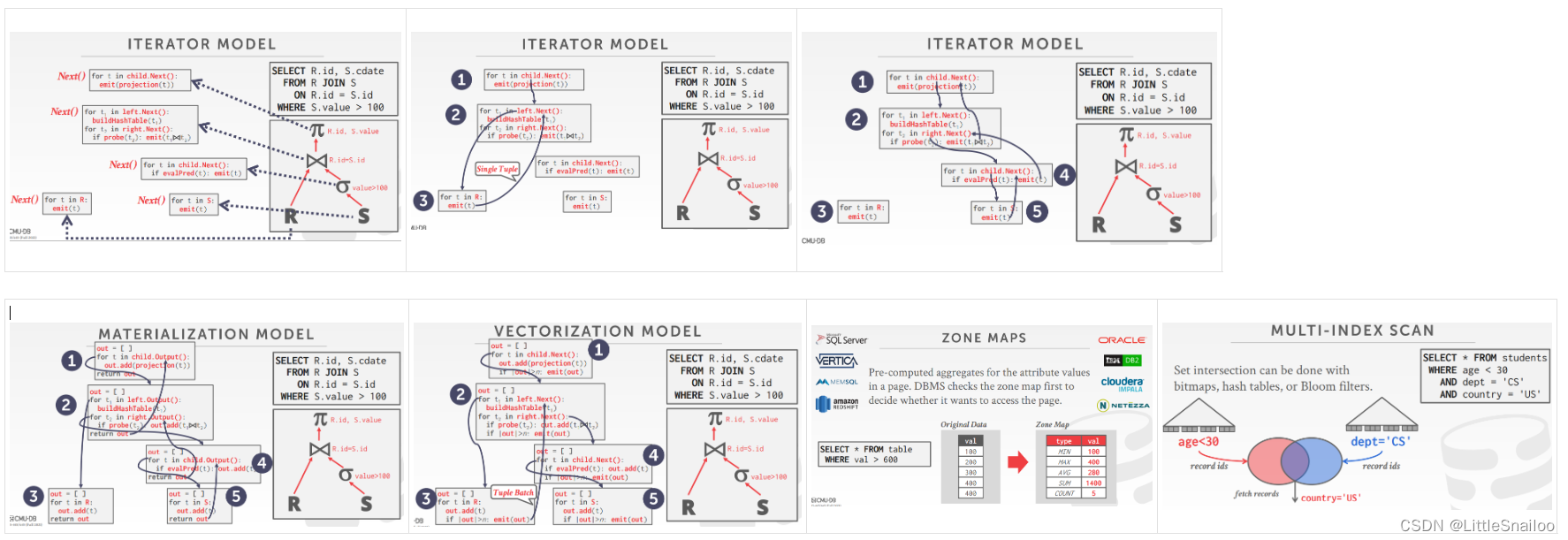
Processing Models 执行模型：定义了系统如何执行一个query plan。主要有以下三个流派：
1. Approach #1: Iterator Model，Also called Volcano or Pipeline Model（火山模型） Each query plan operator implements a Next() function. （单条数据函数调用费时）
2. Approach #2: Materialization Model （物化模型）Each operator processes its input all at once and then emits its output all at once （TP常用）（一次全部结果传递，可能太大）
3. Approach #3: Vectorized / Batch Model （向量模型）Each operator emits a batch of tuples instead of a single tuple （AP常用）Allows for operators to more easily use vectorized (SIMD) instructions to process batches of tuples.
计划执行的方向：（1）自顶向下（2）自底向上
Access Methods： DBMS访问存储在表中的数据的方式
1. Sequential Scan 顺序扫描
  1. 优化的方法：
    1. Prefetching 预读取
    2. Buffer Pool Bypass 以后无用的数据直接在执行器中使用完扔掉不进缓冲池
    3. Parallelization 并行执行
    4. Heap Clustering
    5. Zone Maps 页面中属性值的预计算聚合。DBMS首先检查区域映射，以决定是否要访问页面。增加了磁盘占用及维护成本
    6. Late Materialization 晚物化（列存适用）
2. Index Scan 索引扫描
  1. 使用哪个索引取决于：
    1. What attributes the index contains
    2. What attributes the query references
    3. The attribute's value domains
    4. Predicate composition
    5. Whether the index has unique or non-unique keys
3. Multi-Index / "Bitmap" Scan 多索引/位图扫描
Modification Queries 对数据库有更改的一些查询（增删改）
1. Operators that modify the database (INSERT, UPDATE, DELETE) are responsible for checking constraints and updating indexes.
2. UPDATE/DELETE:
  1. Child operators pass Record IDs for target tuples.
  2. Must keep track of previously seen tuples.(更新或删除时必须记录原来的数据)
3. INSERT:
  1. Materialize tuples inside of the operator.（算子内部物化）
  2. Operator inserts any tuple passed in from child operators.（）
Expression Evaluation
1. The DBMS represents a WHERE clause as an expression tree.
2. The nodes in the tree represent different expression types:
  1. Comparisons (=, , !=)
  2. Conjunction (AND), Disjunction (OR)
  3. Arithmetic Operators (+, -, *, /, %)
  4. Constant Values
  5. Tuple Attribute References

7.Query Executin II 并发

考虑 Parallel Execution 的目的：
1. Increased performance
  1. Throughput：在一个时间单位里可以处理的sql数量（针对多条sql）
  2. Latency：延迟（针对单条sql）
2. Increased responsiveness and availability 提高响应性和可用性
3. Potentially lower total cost of ownership (TCO) 潜在降低总拥有成本(TCO) TCO：硬件成本及使用期间的消耗（如电费等等）总和
Parallel vs. Distributed
1. Parallel DBMSs
  1. Resources are physically close to each other.
  2. Resources communicate over high-speed interconnect.
  3. Communication is assumed to be cheap and reliable.
2. Distributed DBMSs
  1. Resources can be far from each other.
  2. Resources communicate using slow(er) interconnect.
  3. Communication cost and problems cannot be ignored
Process Models：DBMS的进程模型定义了如何设计系统以支持来自多用户应用程序的并发请求。
1. Process per DBMS Worker：每个worker一个进程（频繁创建销毁进程消耗资源）
  1. Relies on OS scheduler.
  2. Use shared-memory for global data structures.
  3. A process crash doesn’t take down entire system.
  4. Examples: IBM DB2, Postgres, Oracle
2. Process Pool 进程池
  1. Still relies on OS scheduler and shared memory.
  2. Bad for CPU cache locality.
  3. Examples: IBM DB2, Postgres (2015)
3. Thread per DBMS Worker 每个worker 一个线程
  1. DBMS manages its own scheduling. 自己调度
  2. May or may not use a dispatcher thread. 有或没有一个分发线程
  3. Thread crash (may) kill the entire system. 影响整个系统
  4. Examples: IBM DB2, MSSQL, MySQL, Oracle (2014)
调度：对于每一个执行计划，数据库需要决定这个执行计划使用多少任务，占用多少cpu资源，结果存储在哪里等等
Execution Parallelism
1. 多条sql并发执行：
  1. 如果所有sql都是只读的，并发将会很少冲突
  2. 如果多条sql都是updating相关的，则涉及事务方面的内容
2. 单条sql并发执行：在每个算子中并发执行：多个线程集中读取数据
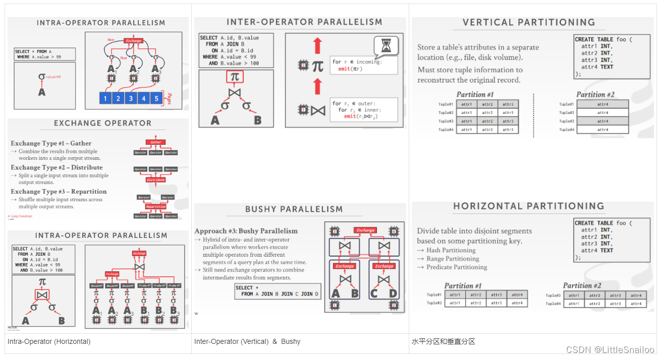
  1. Approach #3: Bushy 1和2的结合: 操作符内部和操作符之间并行性的混合,也需要exchange算子
  2. Approach #2: Inter-Operator (Vertical):Workers execute operators from different segments of a query plan at the same time.Also called pipeline parallelism.
  3. Approach #1: Intra-Operator (Horizontal)：将运算符分解为独立的片段，在不同的数据子集上执行相同的功能。DBMS将一个交换操作符（exchange算子）插入到查询计划中，以合并/分离来自多个子/父操作符的结果
I/O Parallelism：如果磁盘始终是主要瓶颈，使用额外的进程/线程并行执行查询将没有帮助。如果每个worker在磁盘的不同段上工作，情况会变得更糟。所以需要把数据库分开存储在不同的磁盘上
1. Multiple Disks per Database
2. One Database per Disk
3. One Relation per Disk
4. Split Relation across Multiple Disks
Multi-Disk Parallelism：多磁盘并发：硬件层面（RAID磁盘阵列）
分库分区 Partitioning：水平分区和垂直分区

8.Query Optimization 查询优化

sql是声明式的，只声明了需要的结果，具体执行需要优化器选择最优的plan
最早实现的优化器：IBM system 两个流派：直接人为写执行计划 VS. 优化器选择的执行计划
数据库优化器优化的两个流派：
1. Heuristics / Rules 启发式规则
2. Cost-based Search 基于成本的搜索（需要计算等效的多个plan的代价）
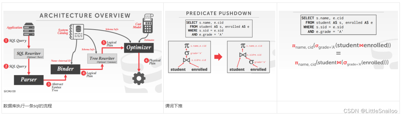
数据库执行一条sql的流程（见下图）
查询优化是 NP-HARD问题
Relational Algebra Equivalences 关系表达式的等价（query rewriting）
1. Predicate Pushdown 谓词下推
2. Perform filters as early as possible 尽可能早的执行过滤器
3. Break a complex predicate, and push down 打破一个复杂的谓词，并向下推 σp1∧p2∧…pn(R) = σp1(σp2(…σpn(R)))
4. 简化复杂谓词 →(x = y and y =3)→x =3 and y =3
5. Inner Join 满足交换律结合律
6. Projections 投影：早物化or晚物化【列存永远晚物化】
7. Projection Pushdown 投影下推
Logical Query Optimization 逻辑查询优化
1. Split Conjunctive Predicates 分离连接谓词
2. Predicate Pushdown 谓词下推（提前筛选数据）
3. Replace Cartesian Products with Joins 用连接代替笛卡尔积
4. Projection Pushdown 投影下推
Nested Queries 嵌套查询的优化
1. Rewrite to de-correlate and/or flatten them 重写
2. Decompose nested query and store result to temporary table 解耦，并存入临时表
Expression Rewriting 表达式的重写
1. 优化器将查询的表达式(例如WHERE子句谓词)转换为最优/最小表达式集。使用if/then/else子句或模式匹配规则引擎实现。搜索匹配模式的表达式，当找到匹配时，重写表达式，如果没有匹配的规则，停止。
Cost Model 代价模型
1. Choice #1: Physical Costs
  1. → Predict CPU cycles, I/O, cache misses, RAM consumption, pre-fetching, etc…
  2. → Depends heavily on hardware.（eg oracle数据库一体机）
2. Choice #2: Logical Costs
  1. → Estimate result sizes per operator. 估计每个算子的结果大小
  2. → Independent of the operator algorithm.每个算子估计开销
  3. → Need estimations for operator result sizes.
3. Choice #3: Algorithmic Costs
  1. → Complexity of the operator algorithm implementation.
基于磁盘的代价模型 cpu io
PG 开销模型：使用CPU和I/O成本的组合，这些成本由“魔法树”常量因素加权。默认设置显然是针对没有大量内存的磁盘驻留数据库:
1. →在内存中处理一个元组比从磁盘读取一个元组快400倍。
2. →顺序I/O比随机I/O快4倍
IBM DB2开销模型
1. 系统目录中的数据库特征
2. 硬件配置
3. 存储器的选择
4. 通信的带宽（分布式）
5. 内存资源
6. 并发相关：用户数、隔离级别、锁的数量

9.Query OptimizationII : Statistics and plan enumeration

More Cost Estimation (Statistics) 统计
1. Manual invocations:
2. → Postgres/SQLite: ANALYZE
3. → Oracle/MySQL: ANALYZE TABLE
4. → SQL Server: UPDATE STATISTICS
5. → DB2: RUNSTATS
For each relation R, the DBMS maintains the following information:
1. → NR: Number of tuples in R.
2. → V(A,R): Number of distinct values for attribute A.
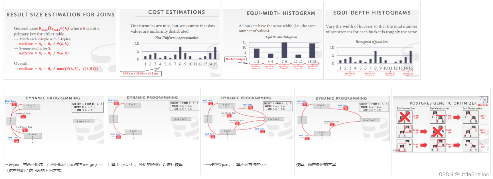
3. SC(A,R)：The selection cardinality SC(A,R) is the average number of records with a value for an attribute A given NR / V(A,R)：选择的基数【假设数据均匀不倾斜】
4. The selectivity (sel) of a predicate P is the fraction of tuples that qualify. sel = SC(P) / NR 谓词P的选择性(sel)是符合条件的元组的百分比。 Formula depends on type of predicate:根据每一个谓词的选择率去计算整体的选择率：
  1. → Equality 相等
  2. → Range 范围
  3. → Negation 不等于
  4. → Conjunction 交集 and
  5. → Disjunction 并集 or
上述公式都基于数据均匀；若数据不均匀，我们可以记录每一种数据的基数，但是这样太耗费空间，解决方式是：直方图 or Sketches（草图）or Sampling
1. 等宽直方图：取相同宽度的数据作为一个bucket，记录每个bucket中的总数。存在的问题：若bucket中各个数据的基数差距很大，统计信息会带来误差。
2. 等深直方图：改变桶的宽度，使每个桶的总出现次数大致相同
3. Sketches: 生成关于数据集的近似统计信息的概率数据结构,成本模型可以用草图代替直方图来提高其选择性估计精度。最常见的例子:
  1. count - min Sketch(1988):一个集合中元素的近似频率计数。
  2. HyperLogLog(2007):一个集合中不同元素的近似数量。（redis）
4. Sampling：现代dbms还从表中收集样本以估计选择性。当底层表发生重大变化时更新示例。（用真实的数据做估计）
Plan Enumeration：在执行基于规则的重写之后，DBMS将为查询列举不同的计划并估计其成本。
1. Single relation.
  1. 单表查询，选择最佳的访问方式：Sequential Scan、Binary Search (clustered indexes)、Index Scan
  2. 【TP型单表查询】OLTP查询的查询计划很容易，因为它们是sargable(Search Argument Able)。→它通常只是选择最好的索引。→连接几乎总是在具有小基数的外键关系上。→可以用简单的启发式方法实现。
2. Multiple relations.
  1. 多表查询，有join的plan有多种，查找最优plan，规定：Fundamental decision in System R: only left-deepjoin trees are considered.（只考虑左深数：可以全部流式计算），可以从以下方面估计代价：
  2. Enumerate the orderings→ Example: Left-deep tree #1, Left-deep tree #2…从不同的join顺序估计
  3. Enumerate the plans for each operator→ Example: Hash, Sort-Merge, Nested Loop…从join使用的不同方法估计
  4. Enumerate the access paths for each table→ Example: Index #1, Index #2, Seq Scan 从访问表使用的不同方法估计
  5. 估计的过程可以采用动态规划降低计算量（见下图）
3. Nested sub-queries.
不同数据库的查询优化：
1. Postgres Optimizer：
  1. Examines all types of join trees→ Left-deep, Right-deep, bushy。join的树有左深树，右深树，综合
  2. Two optimizer implementations:两种优化器实现
    1. → Traditional Dynamic Programming Approach 传统的动态规划方法（小于12个表的join）
    2. → Genetic Query Optimizer (GEQO) 基因遗传算法（大于12个表的join）
  3. Postgres uses the traditional algorithm when # of tables in query is less than 12 and switches to GEQO when there are 12 or more.