MATLAB显函数作图 参数方程作图 极坐标方程作图绘图实例 用 Matlab 绘制高颜值函数图像 放大看告别浓浓锯齿风

1.1  显函数作图

1.2  参数方程作图

1.3  极坐标方程作图

1.1  显函数作图

图1.  

图2.

% Eg001
% fplot 用法
clf
x = linspace(-6,6,10000);
y = sin(pi./x);
subplot(2,1,1)
plot(x,y,'linewidth',0.8)
hold on 
plot([-6 6],[0 0],':r')
axis image
axis equal
grid on
box off
title('\fontsize{16}\it plot 绘制 y = sin (\pi/x)')
xlabel('\fontsize{16}\it x')
ylabel('\fontsize{16}\it y')
subplot(2,1,2)
fplot(@(x) sin(pi./x),[-6,6],'linewidth',0.8)
hold on 
plot([-6 6],[0 0],':r')
axis equal
box off
grid on
title('\fontsize{16}\it fplot 绘制 y = sin (\pi/x)')
xlabel('\fontsize{16}\it x')
ylabel('\fontsize{16}\it y')
% clf
% x = linspace(-3,3,500);
% y = sin(pi./x);
% axis([-3,3,-1.5,1.5])
% plot(x,y,'linewidth',1.5)
% axis equal

% clf
% fplot(@(x) sin(pi./x),[-6,6],'linewidth',0.5)
% axis([-6,6,-1.5,1.5])
%  axis equal
 %axis fill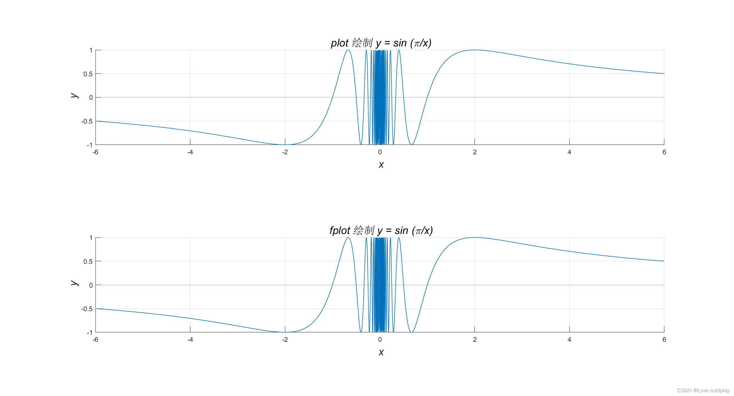

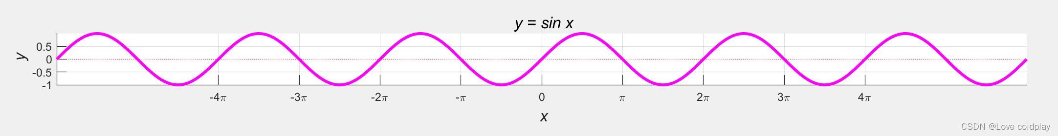
 图 3  y = sinx 6个周期的图像

% Eg002
% sinx
% 6个周期=================================================================================
clf

fplot(@(x) sin(x),[-6*pi,6*pi],'linewidth',2.5,'color','m')%  define, plot

set(gca,'Xtick',[-4*pi,-3*pi,-2*pi,-pi,0,pi,2*pi,3*pi,4*pi],'Ytick',[-1,-0.5,0,0.5,10])% label
set(gca,'XtickLabel',{'-4\pi';'-3\pi';'-2\pi';'-\pi';'0';'\pi';'2\pi';'3\pi';'4\pi'})
set(gca,'YtickLabel',{'-1';'-0.5';'0';'0.5';'1'})

hold on

plot([-6*pi 6*pi],[0 0],':r')% plot

axis equal
box off
grid on
title('\fontsize{14}\it y = sin x')% label
xlabel('\fontsize{14}\it x')
ylabel('\fontsize{14}\it y')


% 2个周期=================================================================================
% clf
% fp=fplot(@(x) sin(x),[-2*pi,2*pi],'linewidth',2.5,'color','m')
% set(gca,'Xtick',[-2*pi,-pi,0,pi,2*pi],'Ytick',[-1,-0.5,0,0.5,10])
% set(gca,'XtickLabel',{'-2\pi';'-\pi';'0';'\pi';'2\pi';})
% set(gca,'YtickLabel',{'-1';'-0.5';'0';'0.5';'1'})
% axis equal
% box off
% grid on
% title('\fontsize{14}\it y = sin x')
% xlabel('\fontsize{14}\it x')
% ylabel('\fontsize{14}\it y')

 1.2  参数方程作图

参数方程作图1

% Eg003
% 参数方程
clf
xt = @(t) cos(9*t);
yt = @(t) sin(10*t);
fplot(xt,yt,'linewidth',1.5)
axis equal square

title('\fontsize{14}\it x = cos 9t, y = sin 10t')

 

 参数方程作图2

% Eg004
% 参数方程2
clf
x =@(t) 2.3*cos (10*t) + cos(23*t);
y =@(t) 2.3*sin (10*t) - sin(23*t);
fplot(x,y,[-3.5,3.5],'linewidth',1,'color','r')
 axis equal square

title('\fontsize{14}\it x = 2.3cos 10t + cos 23t, y = 2.3sin 10t - sin 23t')

 

 1.3  极坐标方程作图

% Eg005
% 极坐标方程

clf

theta = 0:0.01:2*pi;
rho = sin(2*theta).*cos(2*theta);

polarplot(theta,rho,'linewidth',1,'color','r')

title('\fontsize{14}\it r = sin 2\theta cos 2\theta')

 

注意： 如果我们不使用 eps   格式的图片，而是使用其它位图格式的图片例如  png,jpg   等格式，就会出现锯齿：

p

lot

p

2  如何生成 eps 格式的图像？

eps 文件是矢量格式的，矢量格式的图片放大后不会出现锯齿，我们LATEX 中应该使用矢量格式

的图片。

2.1.用matlab绘制好图像后，点击打开图形 (figure) 窗口

2.2.   点击  “File → Save as”

2.3. 在弹出的对话框中选择   “EPS file”   并确定。

函数的基本调用格式为： p

3 如何将Matlab绘制的图片插入TEX文档中？

首先，要将 eps 图片与 TEX 源 文件保存在同一路径下。

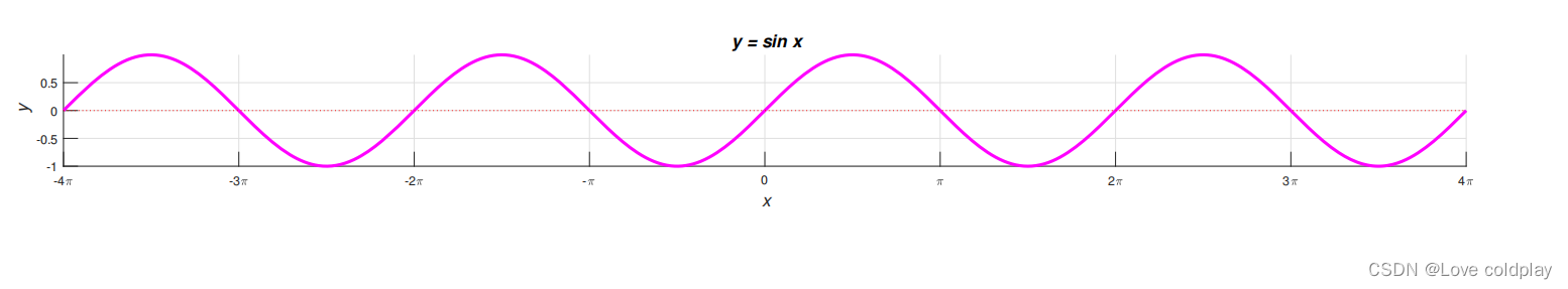
例如，要将 y = sinx 的图片插入到这里，可以用下面的命令：

\begin{figure}[H]
\centering
\includegraphics[width=\textwidth]{sinx4T}
\caption{$y= sin x$\ 4个周期的图像}\label{sinx4t}
\end{figure}

plot(x,y x,y)

)

其中 x

和 y

为长度相同的向量，分别用于存储

x 坐标和

y

坐标

数据

。

p

lot

p

lot

函数的基本调用格式为：

p

plot(

plot(x,y x,y)

)

其中 x

和 y

为长度相同的向量，分别用于存储

x 坐标和

y

坐标

数据

。