Batch Normalization

读者大概率都会遇到这样的情况：模型在训练数据上表现非常好，但无法准确预测测试数据。原因是模型过拟合了，解决此类问题的方法是正则化。

正则化有助于防止模型过度拟合，学习过程变得更加高效。有几个正则化工具：Early Stopping、dropout、权重初始化技术 (Weight Initialization Techniques) 和批量归一化 (Batch Normalization)。

在本文中，将详细探讨批量归一化，内容如下。

• 什么是批量归一化？
• 批量归一化的工作原理？
• 为什么批量归一化有效？
• 如何使用批量归一化？
• PyTorch 简单实现 Batch Normalization

什么是批量归一化？

在进入批量归一化 (Batch Normalization) 之前，让我们了解术语 “Normalization”。归一化是一种数据预处理工具，用于将数值数据调整为通用比例而不扭曲其形状。

通常，当我们将数据输入机器或深度学习算法时，倾向于将值更改为平衡的比例。规范化是为了确保模型可以适当地概括数据。

现在回到 Batch Normalization，这是一个通过在深度神经网络中添加额外层来使神经网络更快、更稳定的过程。新层对来自上一层的层的输入执行标准化和规范化操作。

那批量归一化中术语 “Batch” 是什么？典型的神经网络是使用一组称为 Batch 的输入数据集进行训练的。同样，批归一化中的归一化过程是分批进行的，而不是单个输入。

让我们通过一个例子来理解这一点，我们有一个深度神经网络，如下图所示。

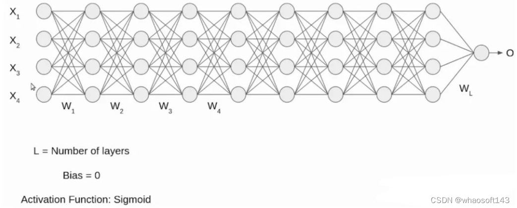
输入 X1、X2、X3、X4 是标准化形式，因为它们来自预处理阶段。当输入通过第一层时，输入 X 和权重矩阵 W 进行点积计算，再经过 sigmoid 函数。以此类推。

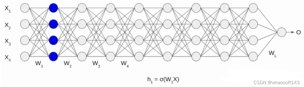
第一层计算方式应用到每一层，最后一层记录为 L，如图所示。 

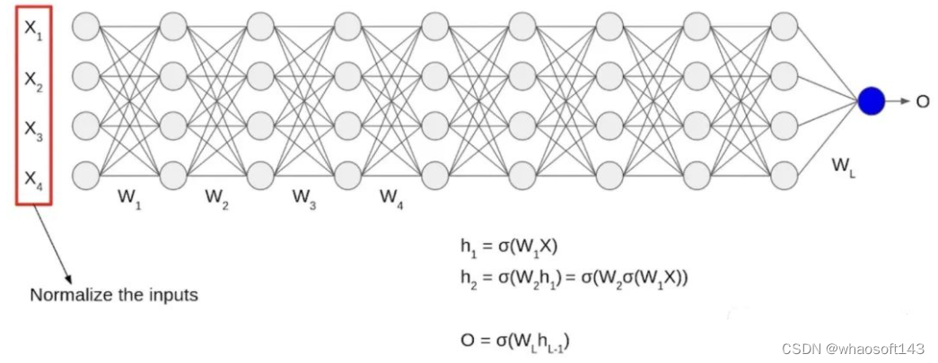
输入 X 随时间归一化，输出将不再处于同一比例。当数据经过多层神经网络并经过 L 个激活函数时，会导致数据发生内部协变量偏移（Internal Covariate Shift）。在深层网络训练的过程中，由于网络中参数变化而引起内部结点数据分布发生变化，这一过程被称作 Internal Covariate Shift。

批量归一化的工作原理？

现在我们对为什么需要批量归一化有了一个清晰的认识，那么让我们了解它是如何工作的。这是一个两步过程。先将输入归一化，然后执行重新缩放和偏移。

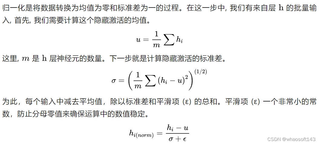
输入的归一化

重新缩放与偏移

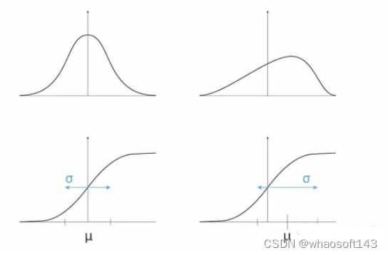
在最后的操作中，将对输入进行重新缩放和偏移。重新缩放参数 γ (gamma) 和偏移参数 β (beta)。

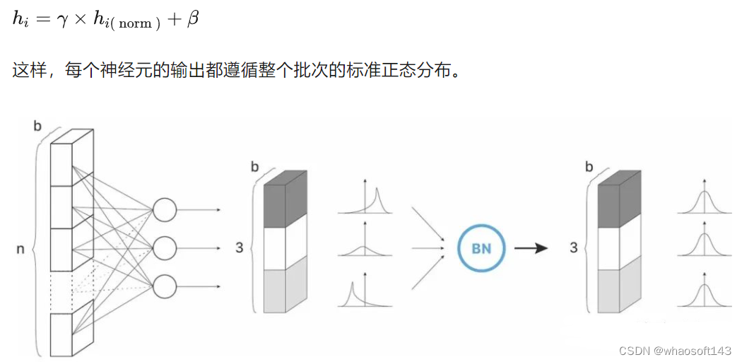
两个可训练参数 𝛾 和 𝛽 应用线性变换来计算层的输出，这样的步骤允许模型通过调整这两个参数来为每个隐藏层选择最佳分布：

• 𝛾 允许调整标准偏差；
• 𝛽 允许调整偏差，在右侧或左侧移动曲线。

为什么批量归一化有效？

在大多数情况下，Batch Normalization 可以提高深度学习模型的性能。那太棒了，但我们想知道黑匣子内部到底发生了什么。在深入讨论之前，我们将看到以下内容：

1. 原始论文 【1】 假设 BN 有效性是减少了内部协变量偏移(ICS)。一篇论文 [2] 驳斥了这一假设。
2. 另一种假设更谨慎地取代了第一种假设：BN 减轻了训练期间各层之间的相互依赖性。
3. 麻省理工学院最近的一篇论文【2】强调了 BN 对优化过程平滑度的影响，使训练更容易。

如果我们要训练一个分类器，判断图片中是否有猫，假设我只有橘猫图片来训练，测试的图片确实是无毛猫。

 

从模型的角度来看，训练图像在统计上与测试图像差异太大，会有一个协变量偏移。

如果输入信号中存在巨大的协变量偏移，优化器将难以很好地泛化。相反，如果输入信号始终服从标准正态分布，优化器将更容易泛化。考虑到这一点，【1】 的作者应用了对隐藏层中的信号进行归一化的策略。他们假设强制 (𝜇 = 0, σ = 1) 中间信号分布将有助于网络在“概念”级别的特征泛化。

但是，我们并不总是希望隐藏单元中的标准正态分布。它会降低模型的代表性。为了解决这个问题，他们添加了两个可训练参数 𝛽 和 𝛾 ，允许优化器为特定任务选择最佳均值（使用 𝛽 ）和标准差（使用 𝛾 ）。

在论文【2】的实验中，训练了三个 VGG 网络（在 CIFAR-10 上）：

• 第一个没有任何 BN 层；
• 第二个确实有 BN 层；
• 第三个与第二个类似，除了他们在激活之前在隐藏单元内明确添加了一些 ICS_distrib （通过添加随机偏差和方差）。

他们测量了每个模型达到的准确度，以及迭代时分布值的演变。这是他们得到的：

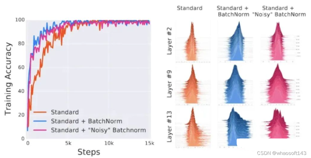
正如预期的那样，我们可以看到第三个网络具有非常高的 ICS。然而，噪声网络的训练速度仍然比标准网络快。其达到的性能可与标准 BN 网络获得的性能相媲美。该结果表明BN 有效性与 ICS_distrib 可能无关。哎呀！

我们不应该过快地抛弃 ICS 理论：如果 BN 有效性不是来自 ICS_distrib，它可能与 ICS 的另一个定义有关。[2] 的作者提出了 ICS 的另一个定义：

We define the internal covariate shift from an optimization perspective as the difference between the gradient computed on a hidden layer k after backpropagating the error L(X)_it, and the gradient computed on the same layer k from the loss L(X)_it+1 computed after the iteration = it update of weights.

看起来好复杂，我们简单的理解一下，这个定义更多地关注梯度而不是隐藏层输入分布，让我们了解 ICS 如何对底层优化问题产生影响。

在下一个实验中，作者记录使用和不使用 BN 层对损失、梯度的影响。让我们来看看结果：

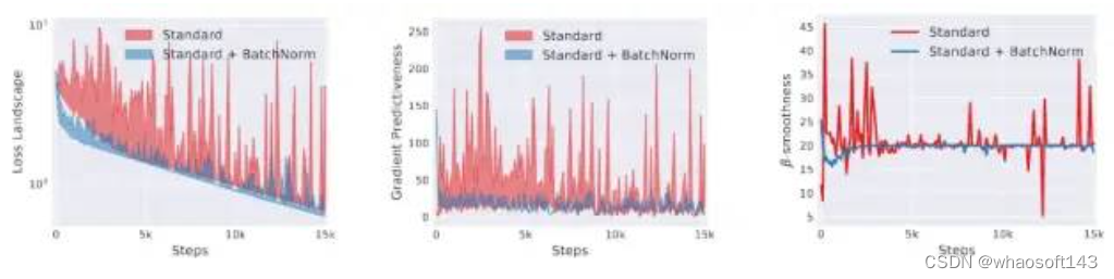
我们可以清楚地看到，使用 BN 层的优化过程更加平滑。

我们终于有了可以用来解释 BN 有效性的结果：BN 层以某种方式使优化更加平滑。这使得优化器的工作更容易：我们可以定义更大的学习率，而不会受到梯度消失（权重卡在突然的平面上）或梯度爆炸（权重突然下降到局部最小值）的影响。

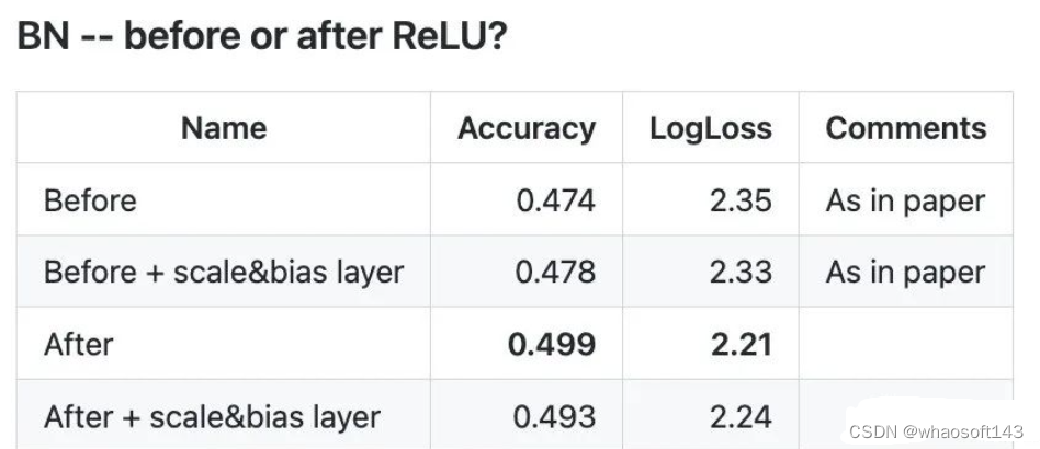
如何使用批量归一化？

之前，BN 层位于非线性函数之前，这与【1】的作者当时的目标和假设是一致的。一些实验表明，将 BN 层放置在非线性函数之后会产生更好的结果【6】。

PyTorch：torch.nn.BatchNorm1d，torch.nn.BatchNorm2d，torch.nn.BatchNorm3d。

Tensorflow/Keras：tf.nn.batch_normalization，tf.keras.layers.BatchNormalization。

torch.nn.BatchNorm2d 示例：

登录后复制

torch.nn.BatchNorm2d(num_features, eps=1e-05, momentum=0.1,   
affine=True, track_running_stats=True, device=None, dtype=None)

• 1.
• 2.

参数如下：
1.num_features：特征的数量,输入一般为 
2.eps：分母中添加的一个常数，为了计算的稳定性，默认为 1e-5；
3.momentum：用于计算 running_mean 和 running_var，默认为 0.1；
4.affine：当为 True 时，会给定可以学习的系数矩阵 gamma 和 beta；
5.track_running_stats：一个布尔值，当设置为 True 时，模型追踪 running_mean 和 running_variance，当设置为 False 时，模型不跟踪统计信息，并在训练和测试时都使用测试数据的均值和方差来代替，默认为 True。

使用 PyTorch 简单实现 Batch Normalization

• 使用 Pytorch 简单实现 BN（应用于 MLP，只有三层隐藏层）；
• 在 MNIST 数据集（一个小的数据集）上测试。

Kaggle 练习网址

复制链接，在 kaggle 平台即可练习：https://www.kaggle.com/code/zymzym/bn-pytorch

• 导入库和设置超参数

登录后复制

# 导入库 Libs  
import numpy as np  
import torch  
from torch import nn  
import torchvision  
import torchvision.datasets as datasets  
from torch.utils.data import DataLoader  
from sklearn.metrics import accuracy_score  
from tqdm.notebook import tqdm  
import matplotlib.pyplot as plt  
  
import warnings  
warnings.filterwarnings('ignore')  
  
# 随机种子 Seeds  
torch.manual_seed(0)  
np.random.seed(0)  
  
# 设置超参数 Hypeparameters  
  
# 两个学习率一样  
LR_BASE = 0.01 # 学习率 lr baseline  
LR_BN = 0.01 # 网络有 BN 的学习率 lr bn network  
  
num_iterations = 10000 # 50000  
valid_steps = 50 # training iterations before validation  
  
verbose = True

• 1.
• 2.
• 3.
• 4.
• 5.
• 6.
• 7.
• 8.
• 9.
• 10.
• 11.
• 12.
• 13.
• 14.
• 15.
• 16.
• 17.
• 18.
• 19.
• 20.
• 21.
• 22.
• 23.
• 24.
• 25.
• 26.
• 27.
• 28.

• 导入 MINST 数据集，本地没有便会下载.

登录后复制

# 导入 MINST 数据集，本地没有便会下载  
  
transform_imgs = torchvision.transforms.Compose([torchvision.transforms.ToTensor(),  
                               torchvision.transforms.Normalize( # Not mentionned in the paper. No normalization  
                                 (0.1307,), (0.3081,))])         # emphasizes the smoothing effect on hidden layers  
                                                                 # activation.  
  
mnist_trainset = datasets.MNIST(root='./data',   
                                train=True,   
                                download=True,   
                                transform=transform_imgs)  
  
mnist_testset = datasets.MNIST(root='./data',   
                               train=False,   
                               download=True,   
                               transform=transform_imgs)  
  
# Dataset loader  
  
train_loader_params = {'shuffle': True, 'batch_size' : 60, 'drop_last' : False}  
test_loader_params = {'shuffle': False, 'batch_size' : 60, 'drop_last' : False}  
  
train_loader = DataLoader(mnist_trainset, **train_loader_params )  
test_loader = DataLoader(mnist_testset, **test_loader_params )  
  
#    每个 batch : (imgs, targets)  
#    图像 : (batch_size=60, channels=1, height=28, width=28) tensor (float32)  
#    标签 : (batch_size=60) tensor (int64)

• 1.
• 2.
• 3.
• 4.
• 5.
• 6.
• 7.
• 8.
• 9.
• 10.
• 11.
• 12.
• 13.
• 14.
• 15.
• 16.
• 17.
• 18.
• 19.
• 20.
• 21.
• 22.
• 23.
• 24.
• 25.
• 26.
• 27.
• 28.

• 复现 BN，遵循一下公式，不熟悉的读者请查看前面的工作原理：

登录后复制

# BatchNorm 复现  
  
class myBatchNorm2d(nn.Module):  
    def __init__(self, input_size = None , epsilon = 1e-3, momentum = 0.99):  
        super(myBatchNorm2d, self).__init__()  
        assert input_size, print('Missing input_size parameter.')  
          
        # 定义训练期间的 Batch 均值和方差  
        self.mu = torch.zeros(1, input_size)  
        # 方差是与平均值的平方偏差的平均值，即 var = mean(abs(x-x.mean())** 2)  
        self.var = torch.ones(1, input_size)  
          
        # 常数，为了数值稳定  
        self.epsilon = epsilon  
          
        # Exponential moving average for mu & var update   
        self.it_call = 0  # training iterations  
        self.momentum = momentum # EMA smoothing  
          
        # 可训练的参数  
        self.beta = torch.nn.Parameter(torch.zeros(1, input_size))  
        self.gamma = torch.nn.Parameter(torch.ones(1, input_size))  
          
        # Batch size on which the normalization is computed  
        self.batch_size = 0  
  
          
    def forward(self, x):  
        # [batch_size, input_size]  
          
        self.it_call += 1  
          
        if self.training :  
              
            if( self.batch_size == 0 ):  
                # First iteration : save batch_size  
                self.batch_size = x.shape[0]  
              
            # Training : compute BN pass  
            batch_mu = (x.sum(dim=0)/x.shape[0]).unsqueeze(0) # [1, input_size]  
            batch_var = (x.var(dim=0)/x.shape[0]).unsqueeze(0) # [1, input_size]  
              
            x_normalized = (x-batch_mu)/torch.sqrt(batch_var + self.epsilon) # [batch_size, input_size]  
            x_bn = self.gamma * x_normalized + self.beta # [batch_size, input_size]  
              
              
            # 更新 mu & std   
            if(x.shape[0] == self.batch_size):  
                running_mu = batch_mu  
                running_var = batch_var  
            else:  
                running_mu = batch_mu*self.batch_size/x.shape[0]  
                running_var = batch_var*self.batch_size/x.shape[0]  
   
            self.mu = running_mu * (self.momentum/self.it_call) + \  
                            self.mu * (1 - (self.momentum/self.it_call))  
            self.var = running_var * (self.momentum/self.it_call) + \  
                        self.var * (1 - (self.momentum/self.it_call))  
              
        else:  
            # 推理 : compute BN pass using estimated mu & var  
            if (x.shape[0] == self.batch_size):  
                estimated_mu = self.mu  
                estimated_var = self.var  
            else :  
                estimated_mu = self.mu*x.shape[0]/self.batch_size  
                estimated_var = self.var*x.shape[0]/self.batch_size  
                  
            x_normalized = (x-estimated_mu)/torch.sqrt(estimated_var + self.epsilon) # [batch_size, input_size]  
            x_bn = self.gamma * x_normalized + self.beta # [batch_size, input_size]  
      
        return x_bn # [batch_size, output_size=input_size]

• 1.
• 2.
• 3.
• 4.
• 5.
• 6.
• 7.
• 8.
• 9.
• 10.
• 11.
• 12.
• 13.
• 14.
• 15.
• 16.
• 17.
• 18.
• 19.
• 20.
• 21.
• 22.
• 23.
• 24.
• 25.
• 26.
• 27.
• 28.
• 29.
• 30.
• 31.
• 32.
• 33.
• 34.
• 35.
• 36.
• 37.
• 38.
• 39.
• 40.
• 41.
• 42.
• 43.
• 44.
• 45.
• 46.
• 47.
• 48.
• 49.
• 50.
• 51.
• 52.
• 53.
• 54.
• 55.
• 56.
• 57.
• 58.
• 59.
• 60.
• 61.
• 62.
• 63.
• 64.
• 65.
• 66.
• 67.
• 68.
• 69.
• 70.
• 71.
• 72.

• 跟踪记录模型的状态。

登录后复制

class ActivationTracker(nn.Module):  
    '''Identity module, which keep track of the current activation during validation.'''  
      
    def __init__(self):  
        super(ActivationTracker, self).__init__()  
  
        # Keep tack of [0.15, 0.5, 0.85] percentiles  
        self.percents_activation_track = [15, 50, 85]  
        self.all_percents_activation = []  
  
    def get_all_activations(self):  
        return np.array(self.all_percents_activation)  
          
    def forward(self, x):  
          
        if not self.training :  
            percents_activation = np.percentile(x.detach().flatten(), self.percents_activation_track)  
            self.all_percents_activation.append(percents_activation)  
            #print('percents_activation = ', percents_activation)  
          
        return x

• 1.
• 2.
• 3.
• 4.
• 5.
• 6.
• 7.
• 8.
• 9.
• 10.
• 11.
• 12.
• 13.
• 14.
• 15.
• 16.
• 17.
• 18.
• 19.
• 20.
• 21.

• 构建 2 个三层隐藏层的网络结构，唯一区别是是否带有 BN。

登录后复制

# 网络结构  
  
def init_weights(model):  
    for module in model:  
        if type(module) == nn.Linear:  
            torch.nn.init.normal_(module.weight, mean=0.0, std=1.0) # "Random Gaussian value"  
            #torch.nn.init.xavier_uniform_(module.weight)  
            module.bias.data.fill_(0.)  
  
  
input_size = 784  
  
# 基准网络  
baseline_model = nn.Sequential(nn.Linear(input_size,100), #1  
                      nn.Sigmoid(),  
                      nn.Linear(100,100), #2  
                      nn.Sigmoid(),  
                      nn.Linear(100,100), #3  
                      ActivationTracker(),  
                      nn.Sigmoid(),  
                      nn.Linear(100,10) # out  
                     )  
  
init_weights(baseline_model)  
  
  
          
# 基准网络带有 BN   
bn_model = nn.Sequential(nn.Linear(input_size,100), #1  
                      myBatchNorm2d(100),  
                      nn.Sigmoid(),  
                      nn.Linear(100,100), #2  
                      myBatchNorm2d(100),  
                      nn.Sigmoid(),  
                      nn.Linear(100,100), #3  
                      myBatchNorm2d(100),  
                      ActivationTracker(),  
                      nn.Sigmoid(),  
                      nn.Linear(100,10) # out  
                     )  
  
init_weights(bn_model)

• 1.
• 2.
• 3.
• 4.
• 5.
• 6.
• 7.
• 8.
• 9.
• 10.
• 11.
• 12.
• 13.
• 14.
• 15.
• 16.
• 17.
• 18.
• 19.
• 20.
• 21.
• 22.
• 23.
• 24.
• 25.
• 26.
• 27.
• 28.
• 29.
• 30.
• 31.
• 32.
• 33.
• 34.
• 35.
• 36.
• 37.
• 38.
• 39.
• 40.
• 41.
• 42.

• 建立训练和测试循环。

登录后复制

# 损失函数 & 评价指标  
criterion = nn.CrossEntropyLoss()  
metric = accuracy_score  
  
  
# 测试循环   
def valid_loop(model, valid_loader, criterion, metric, epoch, verbose = True):  
      
    sum_loss = 0  
    sum_score = 0  
      
    for it, (imgs, targets) in enumerate(valid_loader, start=1):  
        imgs = imgs.view(-1,784)  
          
        with torch.no_grad():  
            out = model(imgs) # [batch_size,num_class]  
            preds  = torch.argmax(out.detach(), dim=1) # [batch_size]  
  
            loss = criterion(out,targets)  
            score = metric(targets, preds)  
  
                      
            sum_loss += loss  
            sum_score += score  
              
    return sum_score/it, sum_loss/it  
  
  
## 训练模型  
def train_loop(model, train_loader, valid_loader, optimizer, scheduler, criterion, metric, verbose = True):  
  
    # 损失函数 & 评价 lists  
    valid_stats = []  
    epochs_valid_stats = []  
  
    with tqdm(range(num_epochs), desc = "Train epochs") as epochs_bar :  
        for e in epochs_bar:  
            # 训练阶段  
            with tqdm(train_loader, leave=False) as it_bar:  
                for it, (imgs, targets) in enumerate(it_bar, start=1):  
                    imgs = imgs.view(-1,784)  
                      
                    out = model(imgs) # [batch_size,num_class]  
                    preds  = torch.argmax(out.detach(), dim=1) # [batch_size]  
                      
                    loss = criterion(out,targets)  
                    score = metric(targets, preds)  
                      
                    optimizer.zero_grad()  
                    loss.backward()  
                    optimizer.step()  
                      
                    if(it % valid_steps == 0):  
                        # 测试阶段  
                        model.eval（)  
                        valid_score, valid_loss = valid_loop(model, valid_loader, criterion, metric, e, verbose)  
                        valid_stats.append([valid_score.astype(np.float32), \  
                                        valid_loss.detach().numpy().astype(np.float32)])  
                        epochs_valid_stats.append(it+e*len(train_loader))  
                          
                        if(verbose):  
                            it_bar.set_postfix(valid_loss=valid_loss.item(), valid_score=valid_score)  
                              
                        model.train()  
                          
                scheduler.step()  
        return np.array(valid_stats), epochs_valid_stats  
              
                      
  
def init_optim_and_scheduler(model, lr = 0.1):  
      
    optimizer = torch.optim.SGD(model.parameters(), lr=lr, momentum=0.9) # momentum not mentioned  
    #optimizer = torch.optim.SGD(model.parameters(), lr=lr)  
    scheduler = torch.optim.lr_scheduler.StepLR(optimizer, step_size=10) # Not mentioned in the paper  
    return optimizer, scheduler  
  
  
      
#---------------------------  
# 训练循环  
#---------------------------  
  
num_epochs = int(num_iterations/len(train_loader))  
  
  
# 没有 BN  
print('-'*15, 'BASELINE MODEL', '-'*15)  
optimizer, scheduler = init_optim_and_scheduler(baseline_model, lr = LR_BASE)  
valid_stats_base, epochs_stats = train_loop(baseline_model, train_loader, test_loader, \  
                                            optimizer, scheduler, criterion, metric, verbose = verbose)  
  
# 有 BN  
print('-'*15, 'BATCH NORMALIZED MODEL', '-'*15)  
optimizer, scheduler = init_optim_and_scheduler(bn_model, lr = LR_BN)  
valid_stats_bn, epochs_stats = train_loop(bn_model, train_loader, test_loader, \  
                                          optimizer, scheduler, criterion, metric, verbose = verbose)

• 1.
• 2.
• 3.
• 4.
• 5.
• 6.
• 7.
• 8.
• 9.
• 10.
• 11.
• 12.
• 13.
• 14.
• 15.
• 16.
• 17.
• 18.
• 19.
• 20.
• 21.
• 22.
• 23.
• 24.
• 25.
• 26.
• 27.
• 28.
• 29.
• 30.
• 31.
• 32.
• 33.
• 34.
• 35.
• 36.
• 37.
• 38.
• 39.
• 40.
• 41.
• 42.
• 43.
• 44.
• 45.
• 46.
• 47.
• 48.
• 49.
• 50.
• 51.
• 52.
• 53.
• 54.
• 55.
• 56.
• 57.
• 58.
• 59.
• 60.
• 61.
• 62.
• 63.
• 64.
• 65.
• 66.
• 67.
• 68.
• 69.
• 70.
• 71.
• 72.
• 73.
• 74.
• 75.
• 76.
• 77.
• 78.
• 79.
• 80.
• 81.
• 82.
• 83.
• 84.
• 85.
• 86.
• 87.
• 88.
• 89.
• 90.
• 91.
• 92.
• 93.
• 94.
• 95.
• 96.
• 97.

• 绘图展示 BN 层在评价指标和损失的影响。

登录后复制

if epochs_stats:   
    fig, ax = plt.subplots(1, 2, figsize=(10*2, 5))  
    #ax.clear()  
      
    # Scores  
    ax[0].plot(epochs_stats, valid_stats_base[:, 0], 'k--', \  
               label = f"Train (baseline) score {valid_stats_base[-1, 0]:.4f}")  
    ax[0].plot(epochs_stats, valid_stats_bn[:, 0], 'b-', \  
               label = f"Train (with BN) score {valid_stats_bn[-1, 0]:.4f}")  
      
    # Losses  
    ax[1].plot(epochs_stats, valid_stats_base[:, 1], 'k--', \  
               label = f"Train (baseline) loss {valid_stats_base[-1, 1]:.4f}")  
    ax[1].plot(epochs_stats, valid_stats_bn[:, 1], 'b-', \  
               label = f"Train (with BN) loss {valid_stats_bn[-1, 1]:.4f}")  
      
    ax[0].legend(); ax[1].legend()  
    plt.show()

• 1.
• 2.
• 3.
• 4.
• 5.
• 6.
• 7.
• 8.
• 9.
• 10.
• 11.
• 12.
• 13.
• 14.
• 15.
• 16.
• 17.
• 18.

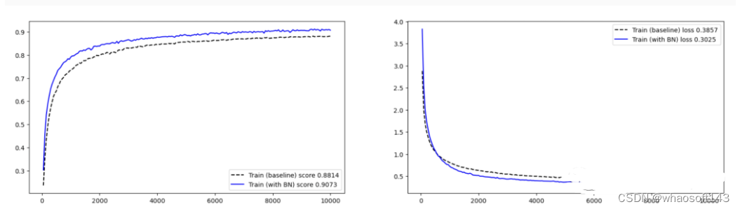
 从实验结果来看，有 BN 的网络，训练的准确率高，收敛更快！

 

原创作者: whaosoft 转载于: https://blog.51cto.com/whaosoft/11639863