TensorFlow2.0学习笔记——常用基础函数

本章内容参考mooc北京大学课程，tensorflow笔记

tf.cast()

• 强制tensor转换为该数据类型

tf.cast(张量名，dtype=数据类型)

tf.reduce_min()

• 计算张量维度上元素的最小值

tf.reduce_min(张量名)

tf.reduce_max()

• 计算张量维度上元素的最大值

tf.reduce_max(张量名)

举例

x1 = tf.constant([1., 2., 3. ],dtype=tf.float32)
print(x1)
# tf.Tensor([1. 2. 3.], shape=(3,), dtype=float32)
x2 = tf.cast(x1, tf.int32)
print(x2)
# tf.Tensor([1 2 3], shape=(3,), dtype=int32)
print(tf.reduce_min(x2),tf.reduce_max(x2))
# tf.Tensor(1, shape=(), dtype=int32) tf.Tensor(3, shape=(), dtype=int32)

axis

在二维张量或数组中，axis=0表示沿第0个方向操作，axis=1表示沿第1个方向操作。在二维张量或数组中，第0个方向是行方向，第1个方向是列方向。

• 沿行方向操作，是指每次操作行下标+1，也就是对一列进行操作
• 沿列方向操作就是对一行进行操作
• 若axis未指定，则对所有数据进行操作。

tf.reduce_mean()

• 计算沿着指定维度的平均值

tf.reduce_mean(张量名， axis=操作轴)

tf.reduce_sum()

• 计算张量沿着指定维度的和

tf.reduce_sum(张量名， axis=操作轴)

举例

x = tf.constant([[1.,2.,3.],
                 [1.,2.,10.]])
print(tf.reduce_mean(x))
# tf.Tensor(3.1666667, shape=(), dtype=float32)
print(tf.reduce_mean(x,axis=1))
# tf.Tensor(3.1666667, shape=(), dtype=float32)

tf.Variable()

• 很重要！！！
• tf.Variable()将变量标记为可训练，如果需要用到梯度下降，一定要使用此函数。
• 被标记的变量会在方向传播中记录梯度信息。
• 神经网络训练中，常用该函数标记带训练参数。

tf.Variable(初始值)

比如：

w = tf.Variable(tf.random.normal([2,2], mean=0,stddev=1))
# 标记一正态分布张量

矩阵乘tf.matmul()

• 实现两个矩阵相乘

a = tf.ones([3,2])
b = tf.fill([2,3], 3.)
print(tf.matmul(b,a))
print(tf.matmul(a,b))

tf.Tensor(
[[9. 9.]
 [9. 9.]], shape=(2, 2), dtype=float32)
tf.Tensor(
[[6. 6. 6.]
 [6. 6. 6.]
 [6. 6. 6.]], shape=(3, 3), dtype=float32)

tf.data.Dataset.from_tensor_slices()

• 将输入特征和标签进行匹配，构建数据集。

data = tf.data.Dataset.from_tensor_slices((输入特征， 标签))

features = tf.constant([12, 23, 10, 17])
labels = tf.constant([0, 1, 1, 0])
dataset = tf.data.Dataset.from_tensor_slices((features, labels))
print(dataset)
for element in dataset:
    print(element)

<TensorSliceDataset shapes: ((), ()), types: (tf.int32, tf.int32)>
(<tf.Tensor: shape=(), dtype=int32, numpy=12>, <tf.Tensor: shape=(), dtype=int32, numpy=0>)
(<tf.Tensor: shape=(), dtype=int32, numpy=23>, <tf.Tensor: shape=(), dtype=int32, numpy=1>)
(<tf.Tensor: shape=(), dtype=int32, numpy=10>, <tf.Tensor: shape=(), dtype=int32, numpy=1>)
(<tf.Tensor: shape=(), dtype=int32, numpy=17>, <tf.Tensor: shape=(), dtype=int32, numpy=0>)

tf.GradientTape()

• 使用with结构记录计算过程，使用gradient求出张量的梯度

with tf.GradientTape() as tape:
    若干个计算过程
   grad = tape.gradient(函数，对谁求导

with tf.GradientTape() as tape:
    w = tf.Variable(tf.constant(3.0))
    loss = tf.pow(w, 2)
grad = tape.gradient(loss, w)
print(grad)

tf.Tensor(6.0, shape=(), dtype=float32)

tf.one_hot()

• 将数据转换为ont_hot矩阵

tf.one_hot(待转换数据， depth=基分类)

• 也可以指定axis

labels = tf.constant([1,0,2])
# 标签为1，0，2
output = tf.one_hot(labels, depth=3)
# 需要注意，这里为三分类，默认标签号只能为0~2，若超过2，则编码为全0
print(output)
output = tf.one_hot(labels, depth=4)
print(output)

tf.Tensor(
[[0. 1. 0.]
 [1. 0. 0.]
 [0. 0. 1.]], shape=(3, 3), dtype=float32)
tf.Tensor(
[[0. 1. 0. 0.]
 [1. 0. 0. 0.]
 [0. 0. 1. 0.]], shape=(3, 4), dtype=float32)

综合应用-鸢尾花分类

• 使用sklearn中的鸢尾花数据集

1.准备数据

# 导入所需模块
import tensorflow as tf
from sklearn import datasets
from matplotlib import pyplot as plt
import numpy as np

# 读入数据
x_data = load_iris().data
y_data = load_iris().target
print(x_data.shape)
# (150, 4)
print(y_data.shape)
# (150,)

# 数据集乱序
# seed: 随机数种子，是一个整数，当设置之后，每次生成的随机数都一样（为方便教学，以保每位同学结果一致）
np.random.seed(116)  # 使用相同的seed，保证输入特征和标签一一对应
np.random.shuffle(x_data)
np.random.seed(116)
np.random.shuffle(y_data)
tf.random.set_seed(116)

# 将打乱后的数据集分割为训练集和测试集，训练集为前120行，测试集为后30行
x_train = x_data[:-30]
y_train = y_data[:-30]
x_test = x_data[-30:]
y_test = y_data[-30:]

# 转换x的数据类型，否则后面矩阵相乘时会因数据类型不一致报错
x_train = tf.cast(x_train, tf.float32)
x_test = tf.cast(x_test, tf.float32)

# from_tensor_slices函数使输入特征和标签值一一对应。（把数据集分批次，每个批次batch组数据）
train_db = tf.data.Dataset.from_tensor_slices((x_train, y_train)).batch(32)
test_db = tf.data.Dataset.from_tensor_slices((x_test, y_test)).batch(32)

2.搭建网络

主要定义神经网络中所有可训练参数。

# 生成神经网络的参数，4个输入特征故，输入层为4个输入节点；因为3分类，故输出层为3个神经元
# 用tf.Variable()标记参数可训练
# 使用seed使每次生成的随机数相同（方便教学，使大家结果都一致，在现实使用时不写seed）
w1 = tf.Variable(tf.random.truncated_normal([4, 3], stddev=0.1, seed=1))
b1 = tf.Variable(tf.random.truncated_normal([3], stddev=0.1, seed=1))

# 设置学习率
lr = 0.1  

train_loss_results = []  # 将每轮的loss记录在此列表中，为后续画loss曲线提供数据
test_acc = []  # 将每轮的acc记录在此列表中，为后续画acc曲线提供数据
epoch = 500  # 循环500轮
loss_all = 0  # 每轮分4个step，loss_all记录四个step生成的4个loss的和

3.训练模型(参数优化)

# 训练部分
for epoch in range(epoch):  #数据集级别的循环，每个epoch循环一次数据集
    for step, (x_train, y_train) in enumerate(train_db):  #batch级别的循环 ，每个step循环一个batch
        with tf.GradientTape() as tape:  # with结构记录梯度信息
            y = tf.matmul(x_train, w1) + b1  # 神经网络乘加运算
            y = tf.nn.softmax(y)  # 使输出y符合概率分布（此操作后与独热码同量级，可相减求loss）
            y_ = tf.one_hot(y_train, depth=3)  # 将标签值转换为独热码格式，方便计算loss和accuracy
            loss = tf.reduce_mean(tf.square(y_ - y))  # 采用均方误差损失函数mse = mean(sum(y-out)^2)
            loss_all += loss.numpy()  # 将每个step计算出的loss累加，为后续求loss平均值提供数据，这样计算的loss更准确
        # 计算loss对各个参数的梯度
        grads = tape.gradient(loss, [w1, b1])

        # 实现梯度更新 w1 = w1 - lr * w1_grad    b = b - lr * b_grad
        w1.assign_sub(lr * grads[0])  # 参数w1自更新
        b1.assign_sub(lr * grads[1])  # 参数b自更新

    # 每个epoch，打印loss信息
    print("Epoch {}, loss: {}".format(epoch, loss_all/4))
    train_loss_results.append(loss_all / 4)  # 将4个step的loss求平均记录在此变量中
    loss_all = 0  # loss_all归零，为记录下一个epoch的loss做准备

    # 测试部分
    # total_correct为预测对的样本个数, total_number为测试的总样本数，将这两个变量都初始化为0
    total_correct, total_number = 0, 0
    for x_test, y_test in test_db:
        # 使用更新后的参数进行预测
        y = tf.matmul(x_test, w1) + b1
        y = tf.nn.softmax(y)
        pred = tf.argmax(y, axis=1)  # 返回y中最大值的索引，即预测的分类
        # 将pred转换为y_test的数据类型
        pred = tf.cast(pred, dtype=y_test.dtype)
        # 若分类正确，则correct=1，否则为0，将bool型的结果转换为int型
        correct = tf.cast(tf.equal(pred, y_test), dtype=tf.int32)
        # 将每个batch的correct数加起来
        correct = tf.reduce_sum(correct)
        # 将所有batch中的correct数加起来
        total_correct += int(correct)
        # total_number为测试的总样本数，也就是x_test的行数，shape[0]返回变量的行数
        total_number += x_test.shape[0]
    acc = total_correct / total_number
    test_acc.append(acc)
    print("Test_acc:", acc)
    print("--------------------------")

• 这一部分输出太多，仅展示开头和结尾的输出

Epoch 0, loss: 0.2821310982108116
Test_acc: 0.16666666666666666
--------------------------
Epoch 1, loss: 0.25459614023566246
Test_acc: 0.16666666666666666
--------------------------
··· ···
··· ···
Epoch 498, loss: 0.03232627175748348
Test_acc: 1.0
--------------------------
Epoch 499, loss: 0.0323002771474421
Test_acc: 1.0
--------------------------

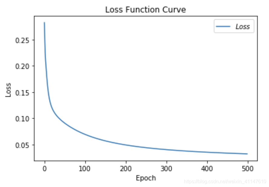
4.训练结果展示

• 模型准确率和损失可视化

# 绘制 loss 曲线
plt.title('Loss Function Curve')  # 图片标题
plt.xlabel('Epoch')  # x轴变量名称
plt.ylabel('Loss')  # y轴变量名称
plt.plot(train_loss_results, label="$Loss$")  # 逐点画出trian_loss_results值并连线，连线图标是Loss
plt.legend()  # 画出曲线图标
plt.show()  # 画出图像

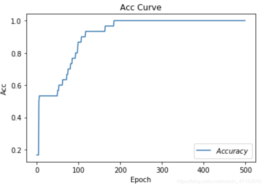
# 绘制 Accuracy 曲线
plt.title('Acc Curve')  # 图片标题
plt.xlabel('Epoch')  # x轴变量名称
plt.ylabel('Acc')  # y轴变量名称
plt.plot(test_acc, label="$Accuracy$")  # 逐点画出test_acc值并连线，连线图标是Accuracy
plt.legend()
plt.show()