Datawhale 零基础入门数据挖掘-Task4 建模调参

Datawhale 零基础入门数据挖掘-Task4 建模调参

四、建模与调参

赛题：零基础入门数据挖掘 - 二手车交易价格预测

1.1 学习目标

• 了解常用的机器学习模型，并掌握机器学习模型的建模与调参流程

1.2 内容介绍

1. 逻辑回归模型
2. 树模型
3. 集成模型
   • 基于bagging思想的集成模型
     • 随机森林模型
     • 随机树模型
   • 基于boosting思想的集成模型
     • XGBOOST
     • LIGHTGBM
     • CATBOOST
     • Adaboost
     • GBDT
   • 基于stacking思想的集成模型
4. 模型对比与性能评估
5. 模型调参
   • 贪心调参方法
   • 网格调参方法
   • 贝叶斯调参方法

1.3 代码实现

1.3.1 读取数据

import pandas as pd
import numpy as np
import warnings
warnings.filterwarnings('ignore')

1.3.2 定义一个减小内存占用的函数：

reduce_mem_usage 函数通过调整数据类型，帮助我们减少数据在内存中占用的空间。

def reduce_mem_usage(df):
    """ iterate through all the columns of a dataframe and modify the data type
        to reduce memory usage.        
    """
    start_mem = df.memory_usage().sum() 
    print('Memory usage of dataframe is {:.2f} MB'.format(start_mem))
    
    for col in df.columns:
        col_type = df[col].dtype
        
        if col_type != object:
            c_min = df[col].min()
            c_max = df[col].max()
            if str(col_type)[:3] == 'int':
                if c_min > np.iinfo(np.int8).min and c_max < np.iinfo(np.int8).max:
                    df[col] = df[col].astype(np.int8)
                elif c_min > np.iinfo(np.int16).min and c_max < np.iinfo(np.int16).max:
                    df[col] = df[col].astype(np.int16)
                elif c_min > np.iinfo(np.int32).min and c_max < np.iinfo(np.int32).max:
                    df[col] = df[col].astype(np.int32)
                elif c_min > np.iinfo(np.int64).min and c_max < np.iinfo(np.int64).max:
                    df[col] = df[col].astype(np.int64)  
            else:
                if c_min > np.finfo(np.float16).min and c_max < np.finfo(np.float16).max:
                    df[col] = df[col].astype(np.float16)
                elif c_min > np.finfo(np.float32).min and c_max < np.finfo(np.float32).max:
                    df[col] = df[col].astype(np.float32)
                else:
                    df[col] = df[col].astype(np.float64)
        else:
            df[col] = df[col].astype('category')

    end_mem = df.memory_usage().sum() 
    print('Memory usage after optimization is: {:.2f} MB'.format(end_mem))
    print('Decreased by {:.1f}%'.format(100 * (start_mem - end_mem) / start_mem))
    return df

这其中，第三行打印中，有**{:.2f}**，这个是指这部分填写后面format(start_mem)的内容，2是指保存两位小数，f是指float类型。
另外，介绍一下：

• np.finfo()
  finfo(dtype)
  显示float类型的机器限制。
  finfo函数是根据dtype类型来获得信息，获得符合这个类型的float型。
• np.iinfo()
  显示整数类型的机器限制。

1.3.3 五折交叉验证 & 模拟真实业务情况

sample_feature['notRepairedDamage'] = sample_feature['notRepairedDamage'].astype(np.float32)
train = sample_feature[continuous_feature_names + ['price']]

train_X = train[continuous_feature_names]
train_y = train['price']

1.3.3- 1 五折交叉验证

在使用训练集对参数进行训练的时候，经常会发现人们通常会将一整个训练集分为三个部分（比如mnist手写训练集）。一般分为：训练集（train_set），评估集（valid_set），测试集（test_set）这三个部分。这其实是为了保证训练效果而特意设置的。其中测试集很好理解，其实就是完全不参与训练的数据，仅仅用来观测测试效果的数据。而训练集和评估集则牵涉到下面的知识了。

因为在实际的训练中，训练的结果对于训练集的拟合程度通常还是挺好的（初始条件敏感），但是对于训练集之外的数据的拟合程度通常就不那么令人满意了。因此我们通常并不会把所有的数据集都拿来训练，而是分出一部分来（这一部分不参加训练）对训练集生成的参数进行测试，相对客观的判断这些参数对训练集之外的数据的符合程度。这种思想就称为交叉验证（Cross Validation）

# 自定义损失函数
def myFeval(preds, xgbtrain):
    label = xgbtrain.get_label()
    score = mean_absolute_error(np.expm1(label), np.expm1(preds))
    return 'myFeval', score, False


param = {'boosting_type': 'gbdt',       
         'num_leaves': 64,
         'max_depth': 10,
         "lambda_l2": 1,  # 防止过拟合
         "lambda_l1": 1,   #  防止过拟合
         'min_data_in_leaf': 20,  # 防止过拟合，好像都不用怎么调
         'objective': 'regression_l1',
         'learning_rate': 0.01,
         "min_child_samples": 20,
         'verbosity': -1,

         "feature_fraction": 0.8,
         "bagging_freq": 1,
         "bagging_fraction": 0.8,
         "bagging_seed": 11,
         "metric": 'mae',
         }
folds = KFold(n_splits=5, shuffle=True, random_state=2020)
oof_lgb = np.zeros(len(X_data))
predictions_lgb = np.zeros(len(X_test))
predictions_train_lgb = np.zeros(len(X_data))
for fold_, (trn_idx, val_idx) in enumerate(folds.split(X_data, Y_data)):
    print("fold n°{}".format(fold_ + 1))
    trn_data = lgb.Dataset(X_data[trn_idx], Y_data[trn_idx])
    val_data = lgb.Dataset(X_data[val_idx], Y_data[val_idx])

    num_round = 50000
    clf = lgb.train(param, trn_data, num_round, valid_sets=[trn_data, val_data], verbose_eval=300,
                    early_stopping_rounds=300, feval=myFeval)
    feature_list_name = clf.feature_name()
    df = pd.DataFrame(feature_list_name, columns=['feature'])
    df['importance'] = list(clf.feature_importance())
    df = df.sort_values(by='importance', ascending=False)
    df.to_csv("feature_importance" + str(fold_) + ".csv", index=False)
    oof_lgb[val_idx] = clf.predict(X_data[val_idx], num_iteration=clf.best_iteration)
    predictions_lgb += clf.predict(X_test, num_iteration=clf.best_iteration) / folds.n_splits
    predictions_train_lgb += clf.predict(X_data, num_iteration=clf.best_iteration) / folds.n_splits

print("lightgbm score: {:<8.8f}".format(mean_absolute_error(np.expm1(oof_lgb), np.expm1(Y_data))))

1.3.3- 2 模拟真实业务情况

但在事实上，由于我们并不具有预知未来的能力，五折交叉验证在某些与时间相关的数据集上反而反映了不真实的情况。通过2018年的二手车价格预测2017年的二手车价格，这显然是不合理的，因此我们还可以采用时间顺序对数据集进行分隔。在本例中，我们选用靠前时间的4/5样本当作训练集，靠后时间的1/5当作验证集，最终结果与五折交叉验证差距不大

import datetime
sample_feature = sample_feature.reset_index(drop=True)
split_point = len(sample_feature) // 5 * 4
train = sample_feature.loc[:split_point].dropna()
val = sample_feature.loc[split_point:].dropna()

train_X = train[continuous_feature_names]
train_y_ln = np.log(train['price'] + 1)
val_X = val[continuous_feature_names]
val_y_ln = np.log(val['price'] + 1)
model = model.fit(train_X, train_y_ln)
mean_absolute_error(val_y_ln, model.predict(val_X))
# 0.19443858353490887

1.3.4 模型调参

在此我们介绍了三种常用的调参方法如下：

• 贪心算法 https://www.jianshu.com/p/ab89df9759c8
• 网格调参 https://blog.csdn.net/weixin_43172660/article/details/83032029
• 贝叶斯调参 https://blog.csdn.net/linxid/article/details/81189154

## LGB的参数集合：

objective = ['regression', 'regression_l1', 'mape', 'huber', 'fair']

num_leaves = [3,5,10,15,20,40, 55]
max_depth = [3,5,10,15,20,40, 55]
bagging_fraction = []
feature_fraction = []
drop_rate = []

1.3.4 - 1 贪心调参

best_obj = dict()
for obj in objective:
    model = LGBMRegressor(objective=obj)
    score = np.mean(cross_val_score(model, X=train_X, y=train_y_ln, verbose=0, cv = 5, scoring=make_scorer(mean_absolute_error)))
    best_obj[obj] = score
    
best_leaves = dict()
for leaves in num_leaves:
    model = LGBMRegressor(objective=min(best_obj.items(), key=lambda x:x[1])[0], num_leaves=leaves)
    score = np.mean(cross_val_score(model, X=train_X, y=train_y_ln, verbose=0, cv = 5, scoring=make_scorer(mean_absolute_error)))
    best_leaves[leaves] = score
    
best_depth = dict()
for depth in max_depth:
    model = LGBMRegressor(objective=min(best_obj.items(), key=lambda x:x[1])[0],
                          num_leaves=min(best_leaves.items(), key=lambda x:x[1])[0],
                          max_depth=depth)
    score = np.mean(cross_val_score(model, X=train_X, y=train_y_ln, verbose=0, cv = 5, scoring=make_scorer(mean_absolute_error)))
    best_depth[depth] = score

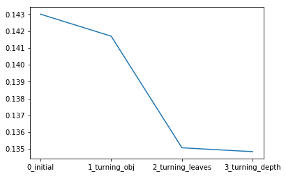
sns.lineplot(x=['0_initial','1_turning_obj','2_turning_leaves','3_turning_depth'], y=[0.143 ,min(best_obj.values()), min(best_leaves.values()), min(best_depth.values())])

1.3.4 - 2 Grid Search 调参

网格调参每次都会浪费很长时间，这里不再做详细介绍，如果想进一步了解网格调参方法，建议阅读： LightGBM调参 - 简书 (jianshu.com)

实际过程中，可先设置一个较大的学习率（如 0.1），通过 LightGBM 原生的 CV 函数确定树个数，之后再通过上述实例代码进行参数调优。最后针对最优的参数设置一个较小的学习率（例如 0.05），同样通过 CV 函数确定树个数，确定最终的参数。注意，针对大数据集，上面每一层参数的调整都需要耗费较长时间。

此外，除 网格搜索 (Grid Search) 外，还有更高效的 随机搜索 (Random Search)，二者的二维超参数搜索空间示例如上图所示，容易理解不再赘述。

1.3.4 - 3 贝叶斯调参

from bayes_opt import BayesianOptimization
def rf_cv(num_leaves, max_depth, min_child_samples,bagging_fraction,feature_fraction,bagging_freq):
    val = cross_val_score(
        LGBMRegressor(objective = 'regression_l1',
            num_leaves=int(num_leaves),
            max_depth=int(max_depth),
            min_child_samples = int(min_child_samples),
            boosting_type = 'gbdt',       
         lambda_l2 = 1,  # 防止过拟合
         lambda_l1 = 1,   #  防止过拟合
         min_data_in_leaf = 20,  # 防止过拟合，好像都不用怎么调
         learning_rate = 0.1,
         verbosity = -1,
        bagging_fraction=round(bagging_fraction, 2), 
        feature_fraction=round(feature_fraction, 2),
        bagging_freq=int(bagging_freq),
         bagging_seed = 11,
         metric = 'mae',
        ),
        X=train_X, y=train_y, verbose=0, cv = 5, scoring=make_scorer(mean_absolute_error)
    ).mean()
    return 1 - val

rf_bo = BayesianOptimization(
    rf_cv,
    {
    'num_leaves': (2, 100),
    'max_depth': (2, 100),
    'min_child_samples' : (2, 100),
    'bagging_fraction':(0.5, 1.0),
    'feature_fraction':(0.5, 1.0),
    'bagging_freq':(0, 100),
    }
)

# 开始优化
rf_bo.maximize(n_iter=10) # 设置迭代次数

1. 贝叶斯调参的主要思想：

给定待优化的目标函数 (广义的函数，只需指定输入和输出即可，无需知道内部结构以及数学性质)，通过不断地添加样本点来更新目标函数的后验分布 (高斯过程，直到后验分布基本贴合于真实分布)，从而选择出最优的超参数以对真实目标函数进行评估。简言之，利用先验知识/基于数据使用贝叶斯定理估计/逼近未知目标函数的后验分布 —— 每次迭代考虑了上一次参数的信息，从而更好的调整当前的参数，然后再根据当前分布选择下一个采样的超参数组合。

2. 贝叶斯优化的基本步骤：

• 初始化一个替代目标函数的概率模型 (高斯过程) —— 代理函数 的先验分布。
• 采样若干数据点 x 使获取函数 a(x) 在当前先验分布上结果最佳。
• 在目标成本函数 c(x) 中评估已采样数据点 x 并获取其输出结果 y。
• 采样新数据点以更新代理函数，得到一个后验分布 (将作为下一步的先验分布)。
• 多次迭代重复第 2-5 步。
• 解读当前的高斯过程分布 (低成本/代价)，找到全局最小值。

总结

在本章中，我们完成了建模与调参的工作，并对我们的模型进行了验证。

1. 集成模型内置的 CV 函数可较快地进行单参数调节，一般可用来优先确定树模型的迭代次数 num_boost_round；
2. 数据量较大时 (如本项目)，网格搜索调参将特别慢，不建议尝试。贝叶斯调参时target值最大的参数组不一定会获得很好的效果，需要取不同的参数组实践才能做判断。

Task4 建模调参 END.