


import sys;
import numpy as np;
import matplotlib.pyplot as plt;
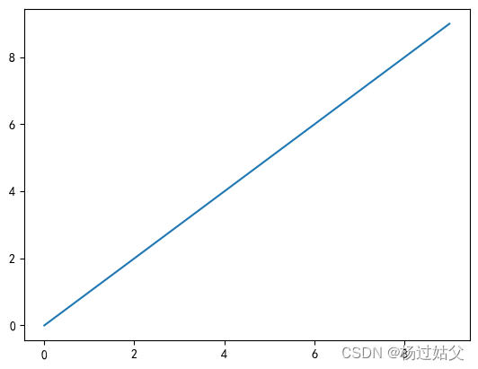
画简单的直线图
In [60]:
arr = np.arange(0 , 10 , 1)
plt.plot(arr , arr)
Out[60]:
[<matplotlib.lines.Line2D at 0x1333b4babf0>]
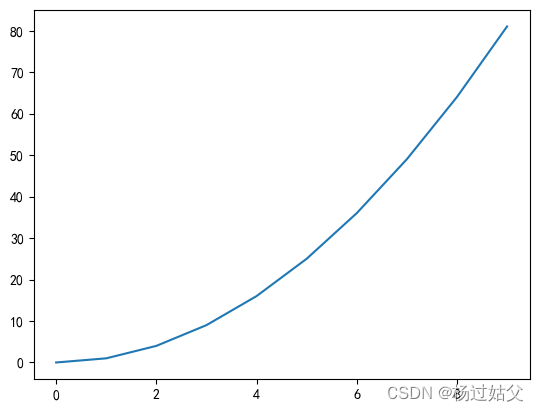
X^2的图
In [61]:
arr = np.arange(0 , 10 , 1)
plt.plot(arr ,  arr**2)
plt.show()
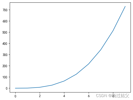
X^2的图
In [63]:
arr = np.arange(0 , 10 , 1)
plt.plot(arr , arr**3)
Out[63]:
[<matplotlib.lines.Line2D at 0x1333b0f2530>]
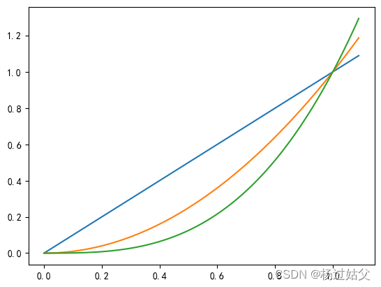
多条线在一个坐标系
In [64]:
arr1 = np.arange(0 , 1.1 , 0.01)
print(arr1)
plt.plot(arr1 , arr1 , arr1 , arr1**2 , arr1 , arr1**3)
[0.   0.01 0.02 0.03 0.04 0.05 0.06 0.07 0.08 0.09 0.1  0.11 0.12 0.13
 0.14 0.15 0.16 0.17 0.18 0.19 0.2  0.21 0.22 0.23 0.24 0.25 0.26 0.27
 0.28 0.29 0.3  0.31 0.32 0.33 0.34 0.35 0.36 0.37 0.38 0.39 0.4  0.41
 0.42 0.43 0.44 0.45 0.46 0.47 0.48 0.49 0.5  0.51 0.52 0.53 0.54 0.55
 0.56 0.57 0.58 0.59 0.6  0.61 0.62 0.63 0.64 0.65 0.66 0.67 0.68 0.69
 0.7  0.71 0.72 0.73 0.74 0.75 0.76 0.77 0.78 0.79 0.8  0.81 0.82 0.83
 0.84 0.85 0.86 0.87 0.88 0.89 0.9  0.91 0.92 0.93 0.94 0.95 0.96 0.97
 0.98 0.99 1.   1.01 1.02 1.03 1.04 1.05 1.06 1.07 1.08 1.09]
Out[64]:
[<matplotlib.lines.Line2D at 0x1333a5be320>,
 <matplotlib.lines.Line2D at 0x1333a5bc670>,
 <matplotlib.lines.Line2D at 0x1333a5bf760>]
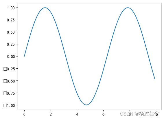
正弦(sin)的图
In [65]:
arr_sin_x = np.arange(0 , 10 , 0.1)
arr_sin_y = np.sin(arr_sin_x)
plt.plot(arr_sin_x , arr_sin_y)
Out[65]:
[<matplotlib.lines.Line2D at 0x1333b1380a0>]
D:\developtools\Python3\lib\site-packages\IPython\core\events.py:82: UserWarning: Glyph 8722 (\N{MINUS SIGN}) missing from current font.
  func(*args, **kwargs)
D:\developtools\Python3\lib\site-packages\IPython\core\pylabtools.py:152: UserWarning: Glyph 8722 (\N{MINUS SIGN}) missing from current font.
  fig.canvas.print_figure(bytes_io, **kw)
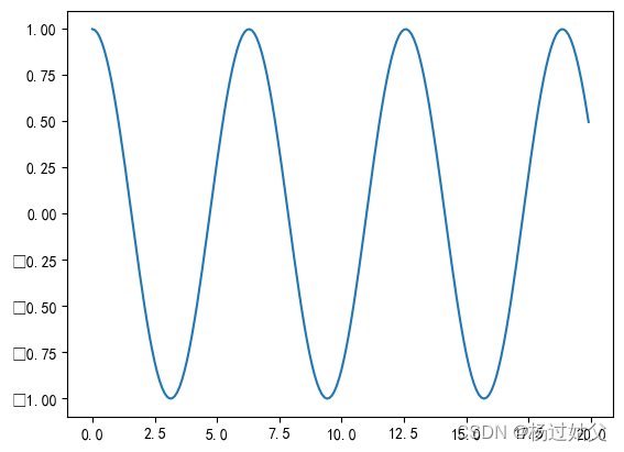
余弦(cos)的图
In [66]:
arr_cos_x = np.arange(0 , 20 , 0.1)
arr_cos_y = np.cos(arr_cos_x)
plt.plot(arr_cos_x , arr_cos_y)
Out[66]:
[<matplotlib.lines.Line2D at 0x13339adeef0>]
In [10]:
days = ['20-06-' + "{:0>2d}".format(x) for x in range(1,31,1)]
days
Out[10]:
['20-06-01',
 '20-06-02',
 '20-06-03',
 '20-06-04',
 '20-06-05',
 '20-06-06',
 '20-06-07',
 '20-06-08',
 '20-06-09',
 '20-06-10',
 '20-06-11',
 '20-06-12',
 '20-06-13',
 '20-06-14',
 '20-06-15',
 '20-06-16',
 '20-06-17',
 '20-06-18',
 '20-06-19',
 '20-06-20',
 '20-06-21',
 '20-06-22',
 '20-06-23',
 '20-06-24',
 '20-06-25',
 '20-06-26',
 '20-06-27',
 '20-06-28',
 '20-06-29',
 '20-06-30']
In [11]:
temps = np.random.uniform(35,39.1,size=(30))
temps
Out[11]:
array([36.91674603, 37.22360246, 35.56612459, 35.81813431, 35.81193556,
       36.52752779, 38.66493055, 35.09208313, 37.27652092, 38.26879424,
       35.63830314, 38.01857516, 38.70259857, 36.57957433, 36.69796371,
       37.22078681, 37.32148446, 37.42713755, 38.06777216, 36.2271336 ,
       38.65586483, 35.67689707, 35.07652181, 35.51593219, 36.15958419,
       37.34306404, 35.96924036, 37.02901597, 38.70485035, 38.01553487])
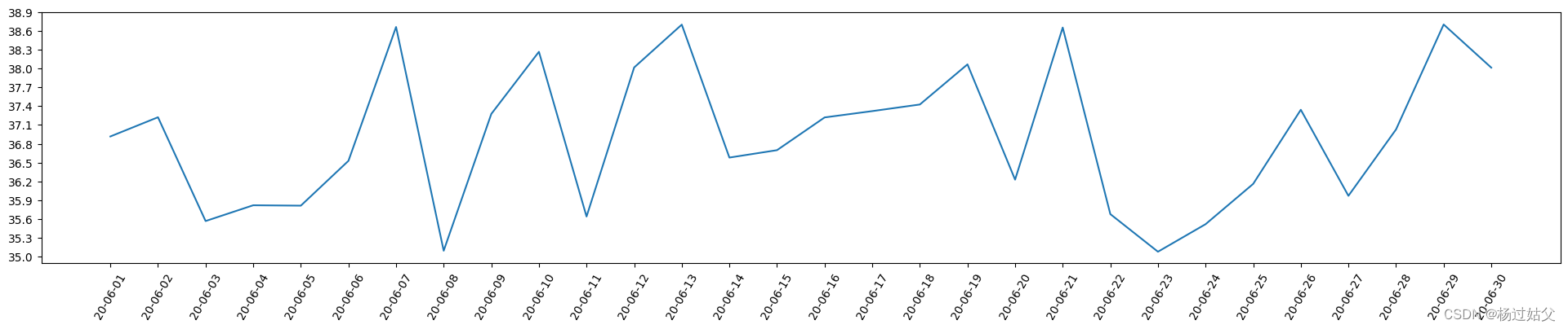
In [12]:
plt.figure(figsize=(24 , 4))
plt.plot(days , temps)
# y 轴添加刻度
plt.yticks([x for x in np.arange(35.0, 39.1, 0.3)])
plt.xticks(rotation=60)
plt.show()
In [13]:
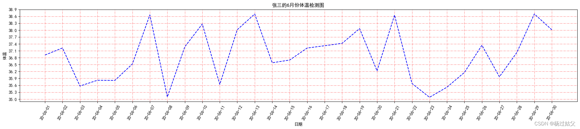
plt.figure(figsize=(24 , 4))
plt.plot(days , temps , '--')
# y 轴添加刻度
plt.yticks([x for x in np.arange(35.0, 39.1, 0.3)])
plt.xticks(rotation=60)
plt.show()

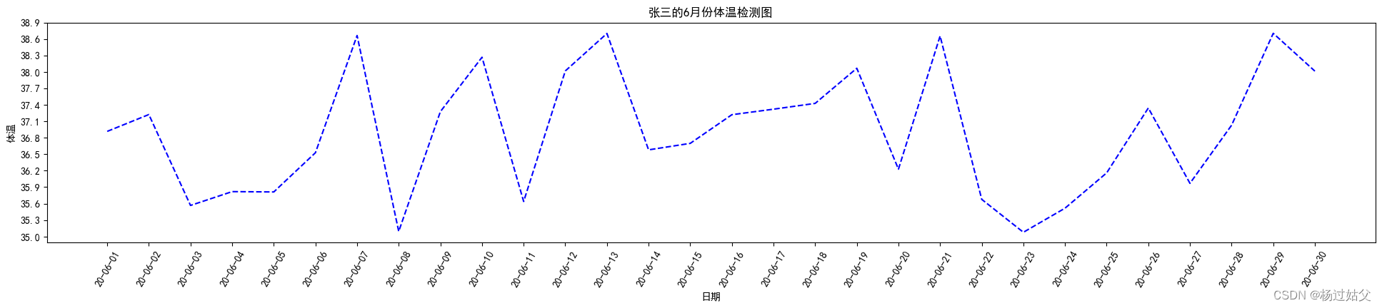
In [14]:
plt.rcParams['font.sans-serif'] = ['SimHei']
plt.figure(figsize=(24 , 4))
# b 代表颜色 blue
plt.plot(days , temps , '--b')
# y 轴添加刻度
plt.yticks([x for x in np.arange(35.0, 39.1, 0.3)])
plt.xticks(rotation=60)
plt.title("张三的6月份体温检测图")
plt.xlabel("日期")
plt.ylabel("体温")
plt.show()
In [15]:
plt.figure(figsize=(24 , 4))
# b 代表颜色 blue
plt.plot(days , temps , '--b')
# y 轴添加刻度
plt.yticks([x for x in np.arange(35.0, 39.1, 0.3)])
plt.xticks(rotation=60)
plt.title("张三的6月份体温检测图")
plt.xlabel("日期")
plt.ylabel("体温")
#linestyle '-', '--', '-.', ':', 'None', ' ', '', 'solid', 'dashed', 'dashdot', 'dotted'
plt.grid(which='major' , axis='both' , linestyle = '-.' , color = 'r' , alpha = 0.5)
plt.show()
In [16]:
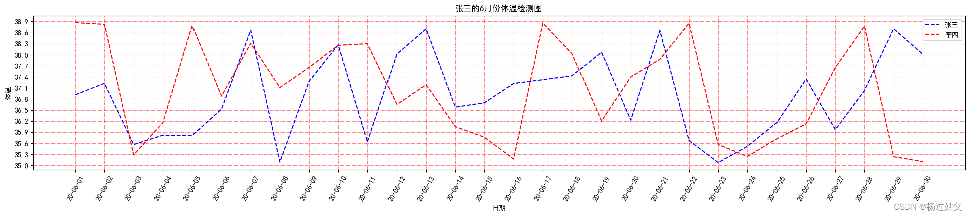
# 使用黑体字体 matplotlib 的默认字体
plt.rcParams['font.sans-serif'] = ['SimHei']

temps1 = np.random.uniform(35,39.1,size=(30))
plt.figure(figsize=(24 , 4))
# b 代表颜色 blue
plt.plot(days , temps , '--b' , label = "张三")
plt.plot(days , temps1 , '--r' , label = "李四")
# y 轴添加刻度
plt.yticks([x for x in np.arange(35.0, 39.1, 0.3)])
plt.xticks(rotation=60)
plt.title("张三的6月份体温检测图")
plt.xlabel("日期")
plt.ylabel("体温")

# which:可以是'major','minor'或'both',表示要显示的网格线的级别。'major'表示主要网格线,'minor'表示次要网格线,'both'表示两者都显示。
# axis:可以是'x','y'或'both',表示要在哪个轴上显示网格线。
#linestyle '-', '--', '-.', ':', 'None', ' ', '', 'solid', 'dashed', 'dashdot', 'dotted'
# color:表示网格线的颜色。
# alpha:表示网格线的透明度,范围是0(完全透明)到1(完全不透明)

plt.grid(which='major' , axis='both' , linestyle = '-.' , color = 'r' , alpha = 0.5)
# 显示图例 前提是在 plt.plot(days , temps , '--b' , label = "张三") 添加了标签 label = "张三"
plt.legend()
plt.show()
In [17]:
plt.rcParams['font.sans-serif'] = ['SimHei']
plt.figure(figsize=(24 , 4))
# b 代表颜色 blue
plt.plot(days , temps , '--b')
# y 轴添加刻度
plt.yticks([x for x in np.arange(35.0, 39.1, 0.3)])
plt.xticks(rotation=60)
plt.title("张三的6月份体温检测图")
plt.xlabel("日期")
plt.ylabel("体温")
plt.show()

In [18]:
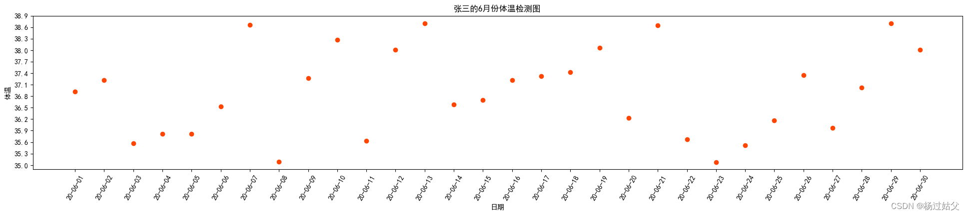
plt.rcParams['font.sans-serif'] = ['SimHei']
plt.figure(figsize=(24 , 4))
# c 颜色

plt.scatter(days , temps , c = '#FF4500')
# y 轴添加刻度
plt.yticks([x for x in np.arange(35.0, 39.1, 0.3)])
plt.xticks(rotation=60)
plt.title("张三的6月份体温检测图")
plt.xlabel("日期")
plt.ylabel("体温")
plt.show()
In [19]:
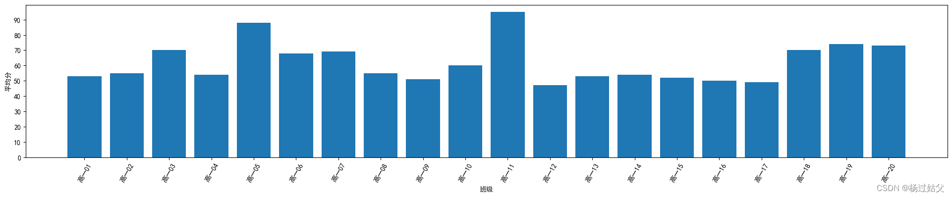
plt.rcParams['font.sans-serif'] = ['SimHei']
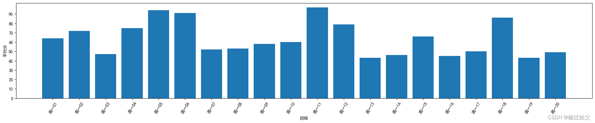
clz_count = 20
avg_score = np.random.randint(40 , 100 , clz_count)
clz = ["高一{:0>2d}".format(x) for x in np.arange(1 , clz_count + 1 , 1)]
plt.figure(figsize=(24 , 4))
plt.xlabel("班级");
plt.ylabel("平均分")
plt.yticks([x for x in np.arange(0 , 100 , 10)])
plt.xticks(rotation = 60)
# 如果 clz 和 avgavg_score 长度不一样 会报下面这个错
# ValueError: shape mismatch: objects cannot be broadcast to a single shape. Mismatch is between arg 0 with shape (19,) and arg 1 with shape (20,)
plt.bar(clz , avg_score)
Out[19]:
<BarContainer object of 20 artists>
In [20]:
plt.rcParams['font.sans-serif'] = ['SimHei']

clz_count = 20
avg_score = np.random.randint(40 , 100 , clz_count)

clz = ["高一{:0>2d}".format(x) for x in np.arange(1 , clz_count + 1 , 1)]

plt.figure(figsize=(24 , 4))
plt.xlabel("班级");
plt.ylabel("平均分")
plt.yticks([x for x in np.arange(0 , 100 , 10)])
plt.xticks(rotation = 60)

# 如果 clz 和 avgavg_score 长度不一样 会报下面这个错
# ValueError: shape mismatch: objects cannot be broadcast to a single shape.  Mismatch is between arg 0 with shape (19,) and arg 1 with shape (20,)
plt.bar(clz , avg_score)
Out[20]:
<BarContainer object of 20 artists>
In [21]:
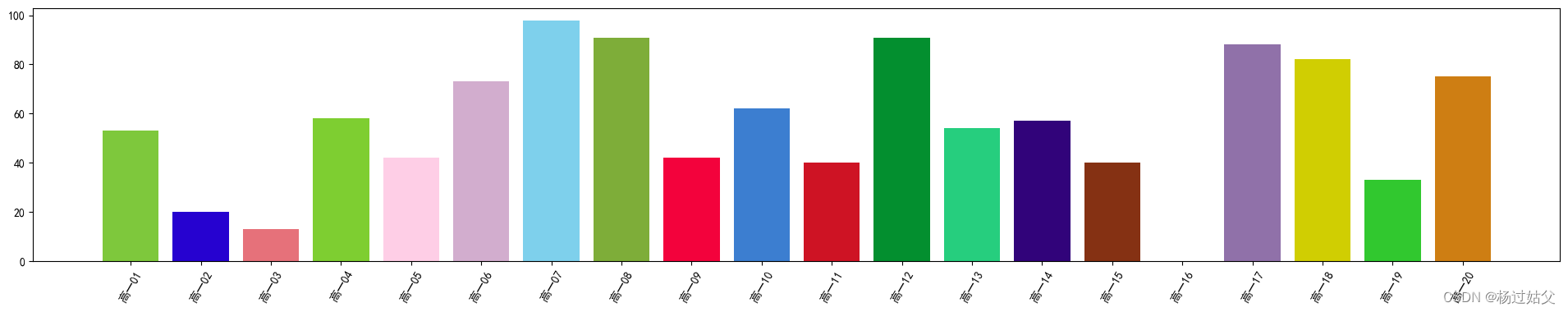
import random

# 生成一个 0-255 的长度位32的数组
c = np.random.randint(0 , 255 , 32)

# 随机从数组 c 中取一个元素
a = random.choice(c)

clz_count = 20
avg_score = np.random.randint(0 , 100 , 20)
clz = ["高一{:0>2d}".format(x) for x in np.arange(1 , 21 , 1)]
colours = ["#{:02x}{:02x}{:02x}".format(random.choice(c) , random.choice(c) , random.choice(c)) for x in np.arange(1 , 21 , 1)]
print(colours)
plt.figure(figsize=(24 , 4))

plt.bar(clz , avg_score , color = colours)

plt.xticks(rotation = 60)
plt.show()
['#7ec83c', '#2602d0', '#e6717a', '#7ece31', '#fecee6', '#d2adce', '#7ed0ec', '#7ead39', '#f3023c', '#3c7ed0', '#ce1324', '#038f2f', '#26ce7e', '#31037a', '#853113', '#a9f390', '#9071a9', '#d0ce02', '#31c82f', '#ce7e13']
In [22]:
import random

# 生成一个 0-255 的长度位32的数组
c = np.random.randint(0 , 255 , 32)

# 随机从数组 c 中取一个元素
a = random.choice(c)

clz_count = 20
avg_score = np.random.randint(0 , 100 , 20)
clz = ["高一{:0>2d}".format(x) for x in np.arange(1 , 21 , 1)]


hexes = [tuple(random.randint(0 , 255) for i in range(3)) for x in range(20)]

colours = ["rgb({0},{1},{2})".format(*c) for c in hexes]


print(colours)
# plt.figure(figsize=(24 , 4))

# plt.bar(clz , avg_score , color = colours)

# lt.xticks(rotation = 60)
# plt.show()
['rgb(191,61,245)', 'rgb(214,86,43)', 'rgb(107,127,65)', 'rgb(248,242,103)', 'rgb(121,160,247)', 'rgb(213,170,74)', 'rgb(103,56,19)', 'rgb(227,237,147)', 'rgb(16,190,121)', 'rgb(56,70,198)', 'rgb(175,116,115)', 'rgb(67,111,245)', 'rgb(249,155,75)', 'rgb(183,23,136)', 'rgb(168,54,227)', 'rgb(58,100,150)', 'rgb(155,102,221)', 'rgb(241,114,22)', 'rgb(232,173,35)', 'rgb(142,153,38)']
In [23]:
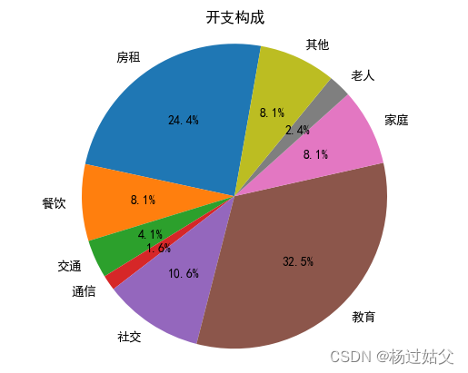
labels = ["房租","餐饮","交通","通信","社交","教育","家庭","老人","其他"]
expend = [30000 , 10000 , 5000 , 2000 , 13000 , 40000 , 10000 , 3000 , 10000 ]
plt.figure()
plt.pie(expend , labels = labels , autopct="%1.1F%%" , shadow=False , startangle=80)
plt.axis("equal")
plt.title("开支构成")
plt.show()
In [24]:
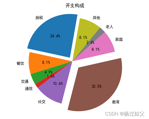
labels = ["房租","餐饮","交通","通信","社交","教育","家庭","老人","其他"]
expend = [30000 , 10000 , 5000 , 2000 , 13000 , 40000 , 10000 , 3000 , 10000 ]
explode = [0.1 , 0 , 0 , 0 , 0 , 0.2 , 0 , 0 , 0]
plt.figure()
plt.pie(expend , labels = labels , autopct="%1.1F%%" , shadow=False , startangle=80 , explode = explode)
plt.axis("equal")
plt.title("开支构成")
plt.show()
In [25]:
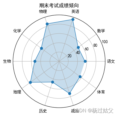
labels = ["语文","数学","英语","物理","化学","生物","地理","历史","政治","体育"]
count = len(labels)
score = np.random.randint(40 , 100 , 9)
# np.concatenate((a, b, c), axis=0) 用于将多个数组按一定规则组合到一起
# 其中,a、b、c是要连接的数组,axis=0表示按列方向连接。

# 为了使雷达图闭合,需要把第一个数据和角度添加到末尾
score = np.concatenate((score , [score[0]]))
print(score)

#  np.linspace 用于在指定的区间内生成等间隔的数值
# numpy.linspace(start, stop, num=50, endpoint=True, retstep=False, dtype=None, axis=0)
# start:序列的起始值。
# stop:序列的终止值。
# num:生成的序列中元素的个数,默认为50。
# endpoint:是否包含终止值,默认为True。
# retstep:如果为True,返回(steps, array),其中steps是生成的序列中每两个相邻元素之间的差值。
# dtype:输出数组的类型。
# axis:在哪个轴上存储生成的数组,默认为0。
# 这里表示生成一个在0到2π之间的等间隔角度数组
angles = np.linspace(0 , 2*np.pi , count , endpoint=False)

# angles = np.concatenate(angles , [angles[0]])
# TypeError: 'list' object cannot be interpreted as an integer 不知道为啥报这个错
# 这样是可以的
# angles = np.concatenate((angles , [angles[0]]))

# 为了使雷达图闭合,需要把第一个数据和角度添加到末尾
#np.append(angles , angles[0])
print(angles)

plt.figure(figsize=(24 , 4))
plt.polar(angles , score , 'o-' , linewidth = 1)
plt.fill(angles , score , alpha=0.25)
plt.title("期末考试成绩倾向")
plt.thetagrids(angles * 180/np.pi , labels)
plt.ylim(0 , 100)
plt.show()
[56 51 95 85 48 53 77 47 73 56]
[0.         0.62831853 1.25663706 1.88495559 2.51327412 3.14159265
 3.76991118 4.39822972 5.02654825 5.65486678]
In [26]:
labels = ["语文","数学","英语","物理","化学","生物","地理","历史","政治","体育"]
count = len(labels)
print(count)
angles = np.linspace(0 , 2*np.pi , count , endpoint=False)
# print(type(angles)) # <class 'numpy.ndarray'>
print(angles)
print(type(angles))

score = np.random.randint(40 , 100 , 9)
# print(type(score)) # <class 'numpy.ndarray'>

# print(type([angles[0]])) #<class 'list'>

# angles = np.concatenate(angles , [angles[0]])
# 以上代码报错 TypeError: 'list' object cannot be interpreted as an integer


# np.array([angles[0]]) 返回的是一个1-d也就是1维的数组  类型是<class 'numpy.ndarray'> 是不能遍历的
# np.array(angles[0]) 返回的是一个0-d也就是0维的数组  但是类型也是<class 'numpy.ndarray'>


bb = np.array([angles[0]] , ndmin = 1)
print(bb)
print(bb[0])
print(type(bb[0]))

a = np.array([[1, 2 , 1], [3, 4 , 3]])
b = np.array([[5, 6 , 5]])
c = np.array([[7, 8]])
print(np.concatenate((a , b)))
print(np.concatenate((a , b), axis = 0) )
print(a)
print(np.concatenate((a , c.T) , axis = 1) )
10
[0.         0.62831853 1.25663706 1.88495559 2.51327412 3.14159265
 3.76991118 4.39822972 5.02654825 5.65486678]
<class 'numpy.ndarray'>
[0.]
0.0
<class 'numpy.float64'>
[[1 2 1]
 [3 4 3]
 [5 6 5]]
[[1 2 1]
 [3 4 3]
 [5 6 5]]
[[1 2 1]
 [3 4 3]]
[[1 2 1 7]
 [3 4 3 8]]
In [35]:
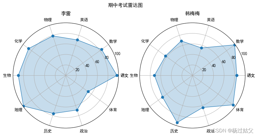
labels = ["语文","数学","英语","物理","化学","生物","地理","历史","政治","体育"]
count = len(labels)
labels1 = np.concatenate((labels , [labels[0]]))
print(labels1)


angles = np.linspace(0 , 2*np.pi , count , endpoint=False)
angles = np.concatenate( (angles , [angles[0]]) )
print(angles)

a_score = np.random.randint(50 , 100 , count)
a_score = np.concatenate((a_score , [a_score[0]]))
print(a_score)


b_score = np.random.randint(50 , 100 , count)
b_score = np.concatenate( (b_score , [b_score[0]]) )
print(b_score)


plt.figure(figsize=(10 , 5))
plt.suptitle("期中考试雷达图")

# 1 , 2 , 1 表示 一行  两列 现在构建的是
plt.subplot(1 , 2 , 1 , projection='polar')
plt.title("李雷")
plt.polar(angles , a_score , 'o-' , linewidth=1)
plt.fill(angles , a_score , alpha=0.25)
plt.thetagrids(angles * 180/np.pi , labels1)
plt.ylim(0 , 100)


plt.subplot(1 , 2 , 2 , projection='polar')
plt.title("韩梅梅")
plt.polar(angles , b_score , 'o-' , linewidth=1)
plt.fill(angles , b_score , alpha=0.25)
plt.thetagrids(angles * 180/np.pi , labels1)
plt.ylim(0 , 100)

plt.show()
['语文' '数学' '英语' '物理' '化学' '生物' '地理' '历史' '政治' '体育' '语文']
[0.         0.62831853 1.25663706 1.88495559 2.51327412 3.14159265
 3.76991118 4.39822972 5.02654825 5.65486678 0.        ]
11
[97 84 71 79 87 90 99 76 69 52 97]
[84 99 55 69 63 72 70 94 64 95 84]
In [32]:
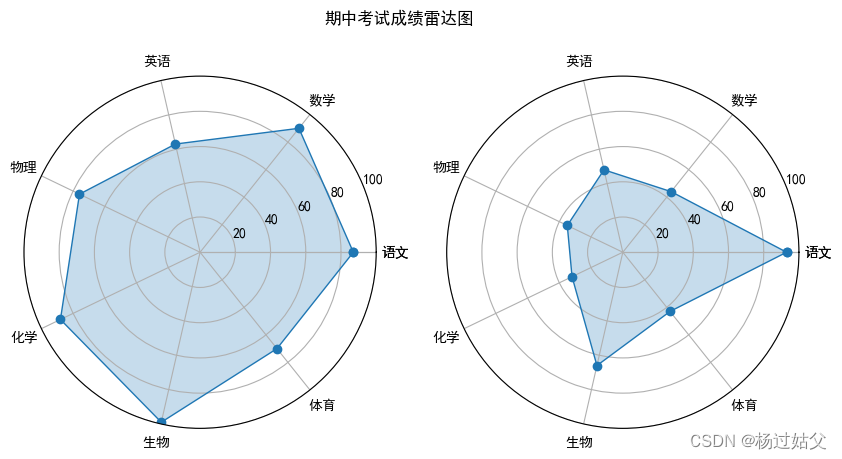
labels = ["语文","数学","英语","物理","化学","生物" , "体育"]
cnt = len(labels)

data1 = [87 , 90 , 63 , 76 , 88 , 99 , 70]
data1 = np.concatenate((data1 , [data1[0]]))
print(data1)

angles = np.linspace(0 , 2*np.pi , cnt , endpoint=False)
angles = np.concatenate((angles, [angles[0]]))
print(angles)


data2 = np.random.randint(30 , 100 , 7)
data2= np.concatenate((data2,[data2[0]]))
print(data2)

plt.figure(figsize=(10 , 5))
plt.suptitle("期中考试成绩雷达图")

labels1 = np.concatenate((labels , [labels[0]]))
print(labels1)

plt.subplot(1, 2, 1 , projection='polar')
plt.polar(angles , data1 , 'o-' , linewidth=1)
plt.fill(angles  , data1 , alpha = 0.25)
plt.thetagrids(angles * 180/np.pi , labels1)
plt.ylim(0 , 100)


plt.subplot(1, 2 , 2 , projection='polar')
plt.polar(angles , data2 , 'o-' , linewidth=1)
plt.fill(angles , data2 , alpha = 0.25)
plt.thetagrids(angles * 180/np.pi , labels1)
plt.ylim(0 , 100)

plt.show()
[87 90 63 76 88 99 70 87]
[0.         0.8975979  1.7951958  2.6927937  3.5903916  4.48798951
 5.38558741 0.        ]
[93 44 48 35 32 66 43 93]
['语文' '数学' '英语' '物理' '化学' '生物' '体育' '语文']
In [36]:
angles = np.linspace(0 , 2*np.pi , count , endpoint=False)
print(angles)
angles = np.linspace(0 , 2*np.pi , count , endpoint=True)
print(angles)
[0.         0.62831853 1.25663706 1.88495559 2.51327412 3.14159265
 3.76991118 4.39822972 5.02654825 5.65486678]
[0.         0.6981317  1.3962634  2.0943951  2.7925268  3.4906585
 4.1887902  4.88692191 5.58505361 6.28318531]
In [40]:
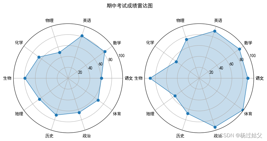
def fill_data(rows , columns ,  index , projection , angles , score , labels):
    plt.subplot(rows , columns , index , projection=projection)
    plt.polar(angles , score , 'o-' , linewidth=1)
    plt.fill(angles , score , alpha = 0.25)
    plt.thetagrids(angles * 180/np.pi , labels)
    plt.ylim(0 , 100)

labels = ["语文","数学","英语","物理","化学","生物","地理","历史","政治","体育"]
count = len(labels)
labels = np.concatenate((labels , [labels[0]]))
print(labels1)


angles = np.linspace(0 , 2*np.pi , count , endpoint=False)
angles = np.concatenate( (angles , [angles[0]]) )
print(angles)

a_score = np.random.randint(50 , 100 , count)
a_score = np.concatenate((a_score , [a_score[0]]))
print(a_score)


b_score = np.random.randint(50 , 100 , count)
b_score = np.concatenate( (b_score , [b_score[0]]) )
print(b_score)

plt.figure(figsize=(10 , 5))
plt.suptitle("期中考试成绩雷达图")

fill_data(1 , 2 , 1 , "polar" , angles , a_score , labels1)
fill_data(1 , 2 , 2 , "polar" , angles , b_score , labels1)

plt.show()
['语文' '数学' '英语' '物理' '化学' '生物' '地理' '历史' '政治' '体育' '语文']
[0.         0.62831853 1.25663706 1.88495559 2.51327412 3.14159265
 3.76991118 4.39822972 5.02654825 5.65486678 0.        ]
[61 83 82 50 66 79 65 71 66 68 61]
[89 91 91 75 52 90 55 68 94 99 89]
In [55]:
fig , axes = plt.subplots(1 , 2 , subplot_kw={'projection': 'polar'})
fig.suptitle("期末考试成绩雷达图")
fig.set_size_inches(10 , 5)

def fill_data(angles , score , labels , sub_title , yLimit , axs):
    print(axs)
    axs.plot(angles , score ,  'o-' , linewidth=1)
    axs.fill(angles , score , alpha = 0.25)
    axs.set_title(sub_title)
    axs.set_thetagrids(angles * 180/np.pi, labels)

labels = ["语文","数学","英语","物理","化学","生物","地理","历史","政治","体育"]
count = len(labels)
labels = np.concatenate((labels , [labels[0]]))

angles = np.linspace(0 , 2*np.pi , count , endpoint=False)
angles = np.concatenate( (angles , [angles[0]]) )

a_score = np.random.randint(50 , 100 , count)
a_score = np.concatenate((a_score , [a_score[0]]))

b_score = np.random.randint(50 , 100 , count)
b_score = np.concatenate( (b_score , [b_score[0]]) )

fill_data(angles , a_score , labels , "张三" , (0 , 100) , axes[0])
fill_data(angles , b_score , labels ,  "李四" , (0 , 100) , axes[1])

plt.show()
PolarAxes(0.125,0.11;0.352273x0.77)
PolarAxes(0.547727,0.11;0.352273x0.77)

In [ ]:


 3608
3608


 被折叠的 条评论
为什么被折叠?
被折叠的 条评论
为什么被折叠?
 到【灌水乐园】发言


