db2实现两个数相减_【Machine Learning】TensorFlow实现K近邻算法预测房屋价格

最新推荐文章于 2022-12-05 16:11:41 发布

余博西

最新推荐文章于 2022-12-05 16:11:41 发布

阅读量384

点赞数

文章标签： db2实现两个数相减

本文链接：https://blog.csdn.net/weixin_42297846/article/details/112323990

版权

来源：AI蜗牛车链接：https://mp.weixin.qq.com/s/XDAv4qKpAYD4ulGNXW7Y-g1前言

机器学习KNN算法(K近邻算法)的总体理论很简单不在这里赘述了。

这篇文章主要问题在于如果利用tensorflow深度学习框架来实现KNN完成预测问题，而不是分类问题，这篇文章中涉及很多维度和思想的转换，希望您可以一步一步跟着我搞定他。

2数据集准备

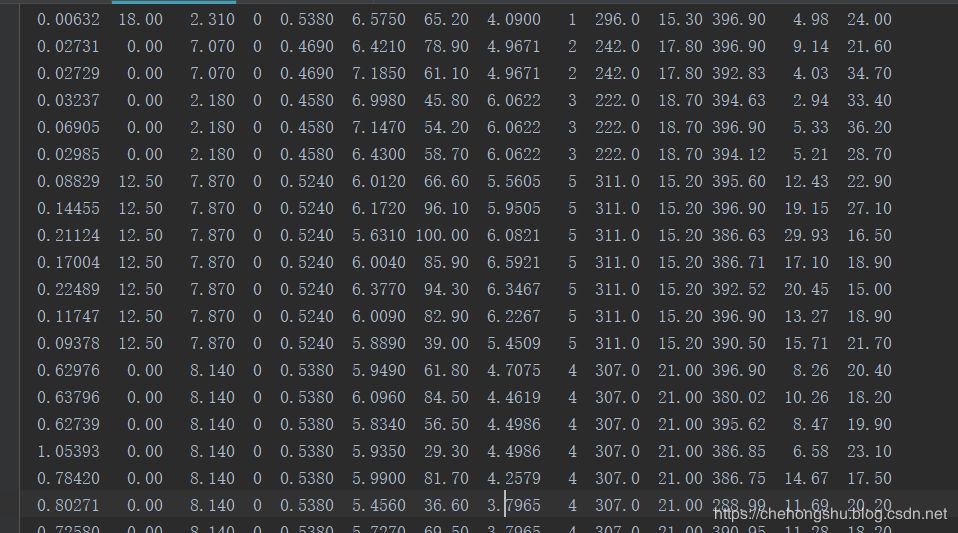
这里使用比较古老的数据集，是房屋预测的数据集

下载地址 https://archive.ics.uci.edu/ml/machine-learning-databases/housing/housing.data

有14列，分别是13个特征，1个房屋价格值

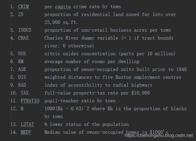
CRIM 村庄的人均犯罪率
ZN 占地面积超过25,000平方尺的住宅用地比例。
INDUS 每个城镇非零售业务的比例
CHAS Charles River虚拟变量(如果管道限制河流则= 1;否则为0)
NOX 一氧化氮浓度(每千万份)
RM 每个居所的平均的屋子数量
AGE 1940年以前建造的自住单位比例
DIS 到波士顿五个就业中心的加权距离
RAD 径向高速公路的可达性指数
TAX 每10,000美元的全额房产税率
PTRATIO 城镇的师生比例
B 城市的黑人比例
LSTAT 人口减少的百分比
MEDV 自住房屋的中位数价值

3数据集预处理

一般对于txt类似的数据集读入都是差不多的步骤

 1path = 'XXX.txt' 2fr = open(path) #打开文件 3lines = fr.readlines() #读入所有行 4dataset = [] 5for line in lines: #遍历每一行(这里的每一行都是string) 6    # 将整个string左右两边的空格和换行符去掉 7    # 可以理解为只保留最外面的两层 8    line = line.strip()  9    # 用空格将string分割成list10    line = line.split('\t')11    # 将list每个元素的string转换为float12    line = [float(i) for i in line]13    dataset.append(line)

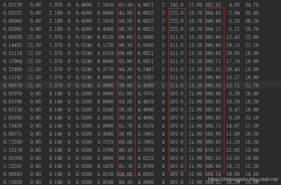
但是这里为.data，其实和txt文件处理相似，由于数据集的每列之间的空格个数不相同，有的是一个空格，有个两个，有的是三个，这里string的split需要用正则化re.split来代替具体代码如下：

1path = 'housing.data'
2fr = open(path)
3lines = fr.readlines()
4dataset = []
5for line in lines:
6    line = line.strip()
7    line = re.split(r' +', line) # re处理
8    line = [float(i) for i in line]
9    dataset.append(line)

这里的feature我们不全都用，只用一部分，因为一些feature与最后的预测没有很密切的关系这里我们采用pandas来进行操作作为容易，还有一点很关键作为特征，有的数大小差距很大，如下图所示：

所标三列就与其他差别很大，这里只是举例，所以需要做归一化处理，利用(data-min)/(max-min)

 1housing_header = ['CRIM', 'ZN', 'INDUS', 'CHAS', 'NOX', 'RM', 'AGE', 'DIS', 'RAD', 'TAX', 'PTRATIO', 'B', 'LSTAT', 'MEDV']
 2# 需要用到的column
 3cols_used = ['CRIM', 'INDUS', 'NOX', 'RM', 'AGE', 'DIS', 'TAX', 'PTRATIO', 'B', 'LSTAT'] 
 4dataset_array = np.array(dataset)
 5# 转换为pandas
 6dataset_pd = pd.DataFrame(dataset_array, columns=housing_header)
 7# 取出特征数据
 8housing_data = dataset_pd.get(cols_used)
 9# 取出房价数据
10labels = dataset_pd.get('MEDV')
11housing_data = np.array(housing_data)
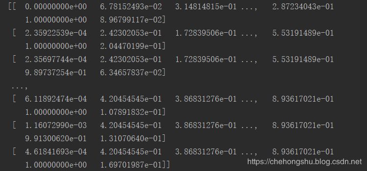
12# 对特征数据进行归一化处理 
13# ptp(0)为每列求出每列数据中的range = max-min
14housing_data = (housing_data - housing_data.min(0))/housing_data.ptp(0)
15# [:, np.newaxis]为行向量转换为列向量
16labels = np.array(labels)[:, np.newaxis]
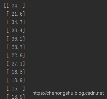
17print(housing_data)
18print(labels)

最终得到的数据为housing_data:

labels:

4训练集和测试集

一般来说训练集和测试集需要随机分配，如果没有验证集的部分，一般为8：2
其实这里可以用sklearn来进行分配操作，但这里我选择用numpy来操作，更为基础写法

 1np.random.seed(22)
 2# 生成随机的index
 3train_ratio = 0.8
 4data_size = len(housing_data)
 5train_index = np.random.choice(a=data_size, size=round(data_size*train_ratio), replace=False)
 6test_index = np.array(list(set(range(data_size))-set(train_index)))
 7# 生成训练集和测试集
 8x_train = housing_data[train_index]
 9y_train = labels[train_index]
10x_test = housing_data[test_index]
11y_test = labels[test_index]

5tensorflow实现KNN

1. 计算图的输入这里不必过多解释， tensorflow的输入x的每一个输入为上面处理之后保留num个features的数据y的每一个输入为加格，即一个数据

1x_train_placeholder = tf.placeholder(tf.float32, [None, num_features])
2x_test_placeholder = tf.placeholder(tf.float32, [None, num_features])
3
4y_train_placeholder = tf.placeholder(tf.float32, [None, 1])
5y_test_placeholder = tf.placeholder(tf.float32, [None, 1])

 2. KNN

2.1 distance实现

故名思议：KNN-K近邻算法既取前k个distance进行判断，如果是classifications问题其实很好判断，只需要选一种计算距离的方式即可，如L2(欧式距离)

也可以是L1

因为此处需要用到tensorflow来编写，需要注意的是矩阵运算，正常来说应该是一个testdata与全部的traindata进行计算，但这里采用bathsize大小的testdata与traindata进行继续，这里集中于矩阵和维度的变换上，先上code再解释 distance计算

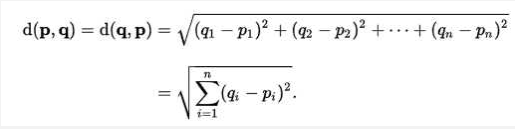
1distance = tf.sqrt(tf.reduce_sum(tf.square(tf.subtract(x_train_placeholder, tf.expand_dims(x_test_placeholder, 1))), reduction_indices=[1]))

这句话其实也可以分解为

1x_test_placeholder_expansion = tf.expand_dims(x_test_placeholder, 1) #增加一个维度
2x_substract = x_train_placeholder - x_test_placeholder_expansion #相减
3x_square = tf.square(x_substract) #平方
4x_square_sum = tf.reduce_sum(x_square, reduction_indices=[1]) # 每个相加
5x_sqrt = tf.sqrt(x_square_sum) # 开方

这几句话主要是做了一个distance计算的过程，就是我们最为熟悉的欧式距离，大概都能看懂，这里主要是讲解两句话

1x_test_placeholder_expansion = tf.expand_dims(x_test_placeholder, 1)

这句话主要是因为这里我们所要做的是每个testdata都与所有的traindata做计算，所以这里需要把testdata扩展一个维度，这样一来就相当于x_train_placeholder - x_test_placeholder_expansion时直接相当于batchsize大小的testdata每一个自己为一个维度的数据都与所有的traindata进行相减。

1x_square_sum = tf.reduce_sum(x_square, reduction_indices=[1]) # 每个相加

这句话做的是将你之前计算出来的每个testdata与所有的traindata计算出来的每个feature之间的相减平方进行相加。

如果以上两句大家实在是无法明白，请自行玩转以下tf的这两个函数即可明白用意。

以上计算距离的方式再预测问题中效果并不好，而是用这里介绍的另一种计算方式L1，代码如下：

1distance = tf.reduce_sum(tf.abs(x_train_placeholder - tf.expand_dims(x_test_placeholder , 1)), axis=2)

2.2 排序实现

因为这里不是分类问题，而是做预测问题，那么问题来了，预测用这个算法怎么做。主要有两种做法。

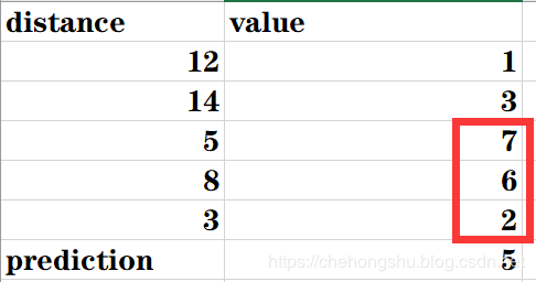
2.2.1 平均权重

每个testdata的预测选择前k个最小的distance，每个distance对应traindata的房价值，做平均值即为预测值，如下图

如果k为3则prediction = (7+6+2)/3 = 5

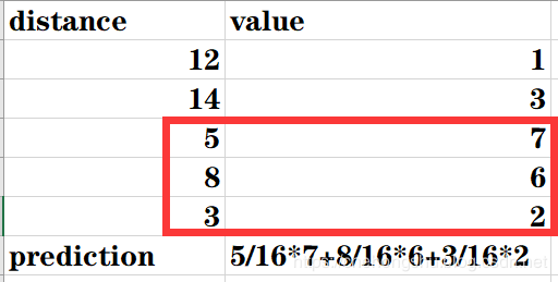
2.2.2 按权重大小来

按权重来，即每个选中的distance作为总共distance总和的比例再乘以此distance对应的value最后求和即可，如下图

这里也有一种编程思想，即如果不乘以7、6、2 剩下那部分其实就有点像前向推理里面的所谓的weights，后面的编程也会如此处理。

2.3 代码实现

 1top_k_value, top_k_index = tf.nn.top_k(tf.negative(distance), k=K)
 2
 3top_k_value = tf.truediv(1.0, top_k_value)
 4
 5top_k_value_sum = tf.reduce_sum(top_k_value, axis=1)
 6top_k_value_sum = tf.expand_dims(top_k_value_sum, 1)
 7top_k_value_sum_again = tf.matmul(top_k_value_sum, tf.ones([1, K], dtype=tf.float32))
 8
 9top_k_weights = tf.div(top_k_value, top_k_value_sum_again)
10weights = tf.expand_dims(top_k_weights, 1)
11
12top_k_y = tf.gather(y_train_placeholder, top_k_index)
13predictions = tf.squeeze(tf.matmul(weights, top_k_y), axis=[1])

这里的代码稍微有点绕，请随着我来一个个看因为tf.topk是返回的前k个的最大的，这里我们要的distance是最小的，所以这里需要对distance来个negative操作也就是取负值

1top_k_value, top_k_index = tf.nn.top_k(tf.negative(distance), k=K)

因为top_k_value变为负数了，所以这里用一个倒数就又可以恢复到以前的大小比较关系了，这里相当于一个数变为负的变小了，再倒数一下，如果所有数都这么干，那最后的大小关系还是之前正数的大小关系，因为我们不需要他的真正大小只需要比例就可以了。倒数代码如下：

1top_k_value = tf.truediv(1.0, top_k_value)

之后开始算整个总和，就可以和前面的公式比对来看，此过程相当于算5+8+3=16的过程

1top_k_value_sum = tf.reduce_sum(top_k_value, axis=1)
2top_k_value_sum = tf.expand_dims(top_k_value_sum, 1)

因为这里我们采用的都是矩阵方式，也就是很多操作需要矩阵化，前面步骤结束之后接下来应该是用每个distace的负数倒数来除以总和sum，但是在相除之前有一个步骤需要进行，相当于为之后的计算做铺垫，，每个sum扩展到k个在一个维度里。

1top_k_value_sum_again = tf.matmul(top_k_value_sum, tf.ones([1, K], dtype=tf.float32))

最后相除

1top_k_weights = tf.div(top_k_value, top_k_value_sum_again)
2weights = tf.expand_dims(top_k_weights, 1)

之后取出前k个value，与整个权重weights进行矩阵相乘计算，前一步的expand_dims和之前仔细讲到的差不多功能，这里不赘述了。

1top_k_y = tf.gather(y_train_placeholder, top_k_index)
2predictions = tf.squeeze(tf.matmul(weights, top_k_y), axis=[1])

3. loss和session

 1loss = tf.reduce_mean(tf.square(tf.subtract(predictions, y_test_placeholder)))
 2
 3loop_nums = int(np.ceil(len(x_test)/batchsize))
 4
 5with tf.Session() as sess:
 6    for i in range(loop_nums):
 7        min_index = i*batchsize
 8        max_index = min((i+1)*batchsize, len(x_test))
 9        x_test_batch = x_test[min_index: max_index]
10        y_test_batch = y_test[min_index: max_index]
11        result, los = sess.run([predictions, loss], feed_dict={
12            x_train_placeholder: x_train, y_train_placeholder: y_train,
13            x_test_placeholder: x_test_batch, y_test_placeholder: y_test_batch
14        })
15
16        print("No.%d batch, loss is %f"%(i+1, los))

loss就为比较常见的计算loss的方式，其他都是tf常用格式，问题不大

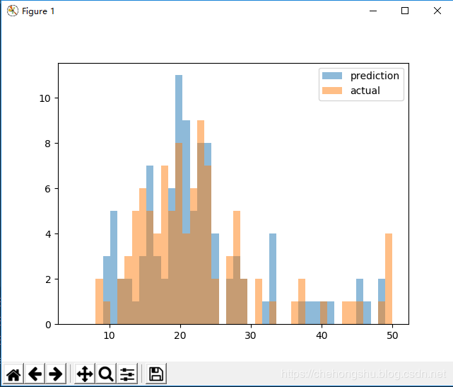
4. 可视化

利用plt可视化柱状图hist

1pins = np.linspace(5, 50, 45)
2print(pins)
3plt.hist(result, pins, alpha=0.5, label='prediction')
4plt.hist(y_test_batch, pins, alpha=0.5, label='actual')
5plt.legend(loc='best')
6plt.show()

5. 全部code

 1import numpy as np
 2import re
 3import pandas as pd
 4import tensorflow as tf
 5from matplotlib import pyplot as plt
 6path = 'housing.data'
 7fr = open(path)
 8lines = fr.readlines()
 9dataset = []
10for line in lines:
11    line = line.strip()
12    line = re.split(r' +', line)
13    line = [float(i) for i in line]
14    dataset.append(line)
15
16housing_header = ['CRIM', 'ZN', 'INDUS', 'CHAS', 'NOX', 'RM', 'AGE', 'DIS', 'RAD', 'TAX', 'PTRATIO', 'B', 'LSTAT', 'MEDV']
17cols_used = ['CRIM', 'INDUS', 'NOX', 'RM', 'AGE', 'DIS', 'TAX', 'PTRATIO', 'B', 'LSTAT']
18dataset_array = np.array(dataset)
19dataset_pd = pd.DataFrame(dataset_array, columns=housing_header)
20housing_data = dataset_pd.get(cols_used)
21labels = dataset_pd.get('MEDV')
22housing_data = np.array(housing_data)
23housing_data = (housing_data - housing_data.min(0))/housing_data.ptp(0)
24labels = np.array(labels)[:, np.newaxis]
25
26np.random.seed(13)
27train_ratio = 0.8
28data_size = len(housing_data)
29train_index = np.random.choice(a=data_size, size=round(data_size*train_ratio), replace=False)
30test_index = np.array(list(set(range(data_size))-set(train_index)))
31
32x_train = housing_data[train_index]
33y_train = labels[train_index]
34x_test = housing_data[test_index]
35y_test = labels[test_index]
36
37num_features = len(cols_used)
38batchsize = len(x_test)
39K = 4
40
41x_train_placeholder = tf.placeholder(tf.float32, [None, num_features])
42x_test_placeholder = tf.placeholder(tf.float32, [None, num_features])
43
44y_train_placeholder = tf.placeholder(tf.float32, [None, 1])
45y_test_placeholder = tf.placeholder(tf.float32, [None, 1])
46
47distance = tf.reduce_sum(tf.abs(tf.subtract(x_train_placeholder, tf.expand_dims(x_test_placeholder, 1))), axis=2)
48
49# distance = tf.sqrt(tf.reduce_sum(tf.square(tf.subtract(x_train_placeholder, tf.expand_dims(x_test_placeholder, 1))), reduction_indices=[1]))
50# x_test_placeholder_expansion = tf.expand_dims(x_test_placeholder, 1)
51# x_substract = x_train_placeholder - x_test_placeholder_expansion
52# x_square = tf.square(x_substract)
53# x_square_sum = tf.reduce_sum(x_square, reduction_indices=[1])
54# x_sqrt = tf.sqrt(x_square_sum)
55
56top_k_value, top_k_index = tf.nn.top_k(tf.negative(distance), k=K)
57
58top_k_value = tf.truediv(1.0, top_k_value)
59
60top_k_value_sum = tf.reduce_sum(top_k_value, axis=1)
61top_k_value_sum = tf.expand_dims(top_k_value_sum, 1)
62top_k_value_sum_again = tf.matmul(top_k_value_sum, tf.ones([1, K], dtype=tf.float32))
63
64top_k_weights = tf.div(top_k_value, top_k_value_sum_again)
65weights = tf.expand_dims(top_k_weights, 1)
66
67top_k_y = tf.gather(y_train_placeholder, top_k_index)
68predictions = tf.squeeze(tf.matmul(weights, top_k_y), axis=[1])
69
70loss = tf.reduce_mean(tf.square(tf.subtract(predictions, y_test_placeholder)))
71
72loop_nums = int(np.ceil(len(x_test)/batchsize))
73
74with tf.Session() as sess:
75    for i in range(loop_nums):
76        min_index = i*batchsize
77        max_index = min((i+1)*batchsize, len(x_test))
78        x_test_batch = x_test[min_index: max_index]
79        y_test_batch = y_test[min_index: max_index]
80        result, los = sess.run([predictions, loss], feed_dict={
81            x_train_placeholder: x_train, y_train_placeholder: y_train,
82            x_test_placeholder: x_test_batch, y_test_placeholder: y_test_batch
83        })
84
85        print("No.%d batch, loss is %f"%(i+1, los))
86
87pins = np.linspace(5, 50, 45)
88print(pins)
89plt.hist(result, pins, alpha=0.5, label='prediction')
90plt.hist(y_test_batch, pins, alpha=0.5, label='actual')
91plt.legend(loc='best')
92plt.show()

6结果

当batchsize为测试数据大小的时候并且k=4

7总结

我们大多数利用KNN都是用分类问题，我们这里为预测方案
我们利用tensorflow深度学习框思想去实现机器学习算法
本实现主要是对KNN以及tensorflow的使用，最为关键是对于矩阵的计算和各种维度变换的更为深刻的使用和理解。

python爬虫人工智能大数据公众号

余博西

关注

0
点赞
踩
0

收藏

觉得还不错? 一键收藏
0
评论
db2实现两个数相减_【Machine Learning】TensorFlow实现K近邻算法预测房屋价格

来源：AI蜗牛车链接：https://mp.weixin.qq.com/s/XDAv4qKpAYD4ulGNXW7Y-g1前言机器学习KNN算法(K近邻算法)的总体理论很简单不在这里赘述了。这篇文章主要问题在于如果利用tensorflow深度学习框架来实现KNN完成预测问题，而不是分类问题，这篇文章中涉及很多维度和思想的转换，希望您可以一步一步跟着我搞定他。2数据集准备这里使用比较...
复制链接

扫一扫