时间序列特征提取：从理论到Python代码实践

时间序列是一种特殊的存在。这意味着你对表格数据或图像进行的许多转换/操作/处理技术对于时间序列来说可能根本不起作用。

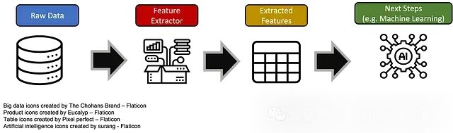
“特征提取"的想法是对我们拥有的数据进行"加工”,确保我们提取所有有意义的特征,以便下一步(通常是机器学习应用)可以从中受益。也就是说它是一种通过提供重要特征并过滤掉所有不太重要的特征来"帮助"机器学习步骤的方法。

这是完整的特征提取过程:

对于表格数据和信号,他们的特征根本就不同，比如说峰和谷的概念,傅里叶变换或小波变换的想法,以及**独立分量分析(ICA)**的概念只有在处理信号时才真正有意义。

目前有两大类进行特征提取的方法:

• 基于数据驱动的方法: 这些方法旨在仅通过观察信号来提取特征。它们忽略机器学习步骤及其目标(例如分类、预测或回归),只看信号,对其进行处理,并从中提取信息。
• 基于模型的方法: 这些方法着眼于整个流程,旨在为特定问题找到解决方案的特征。

数据驱动方法的优点是它们通常在计算上简单易用,不需要相应的目标输出。它们的缺点是特征不是针对你的特定问题的。例如,对信号进行傅里叶变换并将其用作特征可能不如在端到端模型中训练的特定特征那样优化。

在这篇文章中,为了简单起见,我们将只讨论数据驱动方法。并且讨论将基于领域特定的方法**、基于频率的方法、基于时间的方法和基于统计**的方法。

1、领域特定特征提取

提取特征的最佳方法是考虑特定的问题。例如,假设正在处理一个工程实验的信号,我们真正关心的是t = 6s后的振幅。这些是特征提取在一般情况下并不真正有意义,但对特定情况实际上非常相关。这就是我们所说的领域特定特征提取。这里没有太多的数学和编码,但这就是它应该是的样子,因为它极度依赖于你的特定情况。

2、基于频率的特征提取

这种方法与我们的时间序列/信号的谱分析有关。我们有一个自然域，自然域是查看信号的最简单方式,它是时间域,意味着我们将信号视为给定时间的值(或向量)。

例如考虑这个信号,在其自然域中:

绘制它就可以得到:

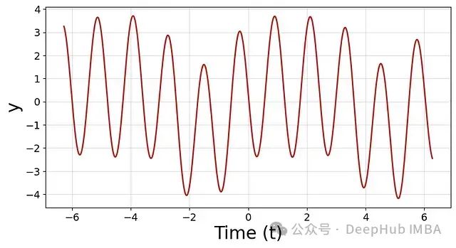
这是自然(时间)域,也是我们数据集的最简单域。

然后我们可以将其转换为频率域。 信号有三个周期性组件。频率域的想法是将信号分解为其周期性组件的频率、振幅和相位。

信号y(t)的傅里叶变换Y(k)如下:

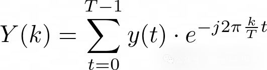
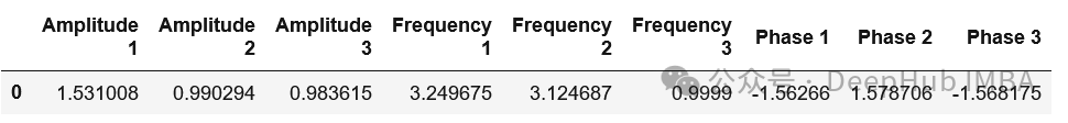
这描述了频率为k的分量的振幅和相位。在提取有意义特征方面,可以提取10个主要分量(振幅最高的)的振幅、相位和频率值。这将是10x3个特征(振幅、频率和相位 x 10),它们将根据谱信息描述时间序列。

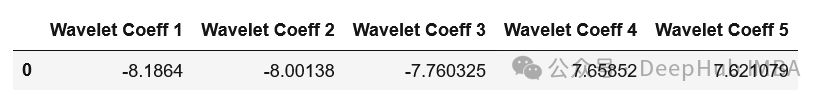
这种方法可以扩展。例如,可以将我们的信号分解,不是基于正弦/余弦函数,而是基于小波,这是另一种形式的周期波。这种分解被称为小波分解。

我们使用代码来详细解释，首先从非常简单的傅里叶变换开始。

首先,我们需要邀请一些朋友来参加派对:

登录后复制

importnumpyasnp
 importmatplotlib.pyplotasplt
 importpandasaspd

• 1.
• 2.
• 3.

现在让我们以这个信号为例:

登录后复制

plt.figure(figsize=(10,5))
 x=np.linspace(-2*np.pi,2*np.pi,1000)
 y=np.sin(x) +0.4*np.cos(2*x) +2*np.sin(3.2*x)
 plt.plot(x,y,color='firebrick',lw=2)
 plt.xlabel('Time (t)',fontsize=24)
 plt.xticks(fontsize=14)
 plt.yticks(fontsize=14)
 plt.grid(alpha=0.4)
 plt.ylabel('y',fontsize=24)

• 1.
• 2.
• 3.
• 4.
• 5.
• 6.
• 7.
• 8.
• 9.

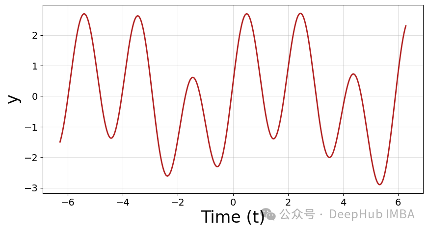
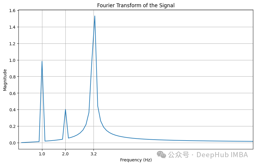
这个信号有三个主要组成部分。一个振幅 = 1和频率 = 1,一个振幅 = 0.4和频率 = 2,一个振幅 = 2和频率 = 3.2。我们可以通过运行傅里叶变换来恢复它们:

登录后复制

importnumpyasnp
 importmatplotlib.pyplotasplt
 
 # Generate the time-domain signal
 x=np.linspace(-8*np.pi, 8*np.pi, 10000)
 y=np.sin(x) +0.4*np.cos(2*x) +2*np.sin(3.2*x)
 y=y-np.mean(y)
 # Perform the Fourier Transform
 Y=np.fft.fft(y)
 # Calculate the frequency bins
 frequencies=np.fft.fftfreq(len(x), d=(x[1] -x[0]) / (2*np.pi))
 # Normalize the amplitude of the FFT
 Y_abs=2*np.abs(Y) /len(x)
 # Zero out very small values to remove noise
 Y_abs[Y_abs<1e-6] =0
 relevant_frequencies=np.where((frequencies>0) & (frequencies<10))
 Y_phase=np.angle(Y)[relevant_frequencies]
 frequencies=frequencies[relevant_frequencies]
 Y_abs=Y_abs[relevant_frequencies]
 
 # Plot the magnitude of the Fourier Transform
 plt.figure(figsize=(10, 6))
 plt.plot(frequencies, Y_abs)
 plt.xlim(0, 10)  # Limit x-axis to focus on relevant frequencies
 plt.xticks([3.2,1,2])
 plt.title('Fourier Transform of the Signal')
 plt.xlabel('Frequency (Hz)')
 plt.ylabel('Magnitude')
 plt.grid(True)
 plt.show()

• 1.
• 2.
• 3.
• 4.
• 5.
• 6.
• 7.
• 8.
• 9.
• 10.
• 11.
• 12.
• 13.
• 14.
• 15.
• 16.
• 17.
• 18.
• 19.
• 20.
• 21.
• 22.
• 23.
• 24.
• 25.
• 26.
• 27.
• 28.
• 29.
• 30.

我们可以清楚地看到三个峰值,对应的振幅和频率。

可以用一个非常简单的函数来完成所有工作

登录后复制

defextract_fft_features( y, x=None,  num_features=5,max_frequency=10):
   y=y-np.mean(y)
   # Perform the Fourier Transform
   Y=np.fft.fft(y)
   # Calculate the frequency bins
   ifxisNone:
     x=np.linspace(0,len(y))
   frequencies=np.fft.fftfreq(len(x), d=(x[1] -x[0]) / (2*np.pi))
   Y_abs=2*np.abs(Y) /len(x)
   Y_abs[Y_abs<1e-6] =0
   relevant_frequencies=np.where((frequencies>0) & (frequencies<max_frequency))
   Y_phase=np.angle(Y)[relevant_frequencies]
   frequencies=frequencies[relevant_frequencies]
   Y_abs=Y_abs[relevant_frequencies]
   largest_amplitudes=np.flip(np.argsort(Y_abs))[0:num_features]
   top_5_amplitude=Y_abs[largest_amplitudes]
   top_5_frequencies=frequencies[largest_amplitudes]
   top_5_phases=Y_phase[largest_amplitudes]
   fft_features=top_5_amplitude.tolist()+top_5_frequencies.tolist()+top_5_phases.tolist()
   amp_keys= ['Amplitude '+str(i) foriinrange(1,num_features+1)]
   freq_keys= ['Frequency '+str(i) foriinrange(1,num_features+1)]
   phase_keys= ['Phase '+str(i) foriinrange(1,num_features+1)]
   fft_keys=amp_keys+freq_keys+phase_keys
   fft_dict= {fft_keys[i]:fft_features[i] foriinrange(len(fft_keys))}
   fft_data=pd.DataFrame(fft_features).T
   fft_data.columns=fft_keys
   returnfft_dict, fft_data

• 1.
• 2.
• 3.
• 4.
• 5.
• 6.
• 7.
• 8.
• 9.
• 10.
• 11.
• 12.
• 13.
• 14.
• 15.
• 16.
• 17.
• 18.
• 19.
• 20.
• 21.
• 22.
• 23.
• 24.
• 25.
• 26.
• 27.

所以如果输入信号y和(可选):

• x或时间数组，考虑的特征数量(或峰值)，最大频率

输出:

登录后复制

x=np.linspace(-8*np.pi, 8*np.pi, 10000)
 y=np.sin(x) +0.4*np.cos(2*x) +2*np.sin(3.2*x)
 extract_fft_features(x=x,y=y,num_features=3)[1]

• 1.
• 2.
• 3.

如果想使用**小波(不是正弦/余弦)***来提取特征,可以进行小波变换。需要安装这个库:

登录后复制

pip install PyWavelets

• 1.

然后运行这个:

登录后复制

importnumpyasnp
 importpywt
 importpandasaspd
 
 defextract_wavelet_features(y, wavelet='db4', level=3, num_features=5):
     y=y-np.mean(y)  # Remove the mean
 
     # Perform the Discrete Wavelet Transform
     coeffs=pywt.wavedec(y, wavelet, level=level)
 
     # Flatten the list of coefficients into a single array
     coeffs_flat=np.hstack(coeffs)
 
     # Get the absolute values of the coefficients
     coeffs_abs=np.abs(coeffs_flat)
 
     # Find the indices of the largest coefficients
     largest_coeff_indices=np.flip(np.argsort(coeffs_abs))[0:num_features]
 
     # Extract the largest coefficients as features
     top_coeffs=coeffs_flat[largest_coeff_indices]
 
     # Generate feature names for the wavelet features
     feature_keys= ['Wavelet Coeff '+str(i+1) foriinrange(num_features)]
 
     # Create a dictionary for the features
     wavelet_dict= {feature_keys[i]: top_coeffs[i] foriinrange(num_features)}
 
     # Create a DataFrame for the features
     wavelet_data=pd.DataFrame(top_coeffs).T
     wavelet_data.columns=feature_keys
 
     returnwavelet_dict, wavelet_data
 
 # Example usage:
 wavelet_dict, wavelet_data=extract_wavelet_features(y)
 wavelet_data

• 1.
• 2.
• 3.
• 4.
• 5.
• 6.
• 7.
• 8.
• 9.
• 10.
• 11.
• 12.
• 13.
• 14.
• 15.
• 16.
• 17.
• 18.
• 19.
• 20.
• 21.
• 22.
• 23.
• 24.
• 25.
• 26.
• 27.
• 28.
• 29.
• 30.
• 31.
• 32.
• 33.
• 34.
• 35.
• 36.
• 37.

3.、基于统计的特征提取

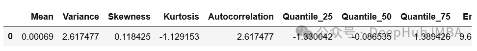
特征提取的另一种方法是依靠统计学。 给定一个信号,有多种方法可以从中提取一些统计信息。从简单到复杂,这是我们可以提取的信息列表:

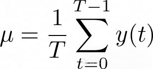
• 平均值,只是信号的总和除以信号的时间步数。

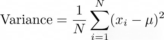
• 方差,即信号与平均值的偏离程度:

• 偏度和峰度。这些是测试你的时间序列分布"不是高斯分布"程度的指标。偏度描述它有多不对称,峰度描述它有多"拖尾"。
• 分位数:这些是将时间序列分成具有概率范围的区间的值。例如,0.25分位数值为10意味着你的时间序列中25%的值低于10,剩余75%大于10
• 自相关。这基本上告诉你时间序列有多"模式化",意味着时间序列中模式的强度。或者这个指标表示时间序列值与其自身过去值的相关程度。
• 熵:表示时间序列的复杂性或不可预测性。

这些属性中的每一个都可以用一行代码实现:

登录后复制

importnumpyasnp
 importpandasaspd
 fromscipy.statsimportskew, kurtosis
 
 defextract_statistical_features(y):
     defcalculate_entropy(y):
         # Ensure y is positive and normalized
         y=np.abs(y)
         y_sum=np.sum(y)
 
         # Avoid division by zero
         ify_sum==0:
             return0
 
         # Normalize the signal
         p=y/y_sum
 
         # Calculate entropy
         entropy_value=-np.sum(p*np.log2(p+1e-12))  # Add a small value to avoid log(0)
 
         returnentropy_value
     # Remove the mean to center the data
     y_centered=y-np.mean(y)
     y=y+np.max(np.abs(y))*10**-4
 
     # Statistical features
     mean_value=np.mean(y)
     variance_value=np.var(y)
     skewness_value=skew(y)
     kurtosis_value=kurtosis(y)
     autocorrelation_value=np.correlate(y_centered, y_centered, mode='full')[len(y) -1] /len(y)
     quantiles=np.percentile(y, [25, 50, 75])
     entropy_value=calculate_entropy(y)  # Add a small value to avoid log(0)
 
     # Create a dictionary of features
     statistical_dict= {
         'Mean': mean_value,
         'Variance': variance_value,
         'Skewness': skewness_value,
         'Kurtosis': kurtosis_value,
         'Autocorrelation': autocorrelation_value,
         'Quantile_25': quantiles[0],
         'Quantile_50': quantiles[1],
         'Quantile_75': quantiles[2],
         'Entropy': entropy_value
     }
 
     # Convert to DataFrame for easy visualization and manipulation
     statistical_data=pd.DataFrame([statistical_dict])
 
     returnstatistical_dict, statistical_data
 
 y=np.sin(x) +0.4*np.cos(2*x) +2*np.sin(3.2*x)
 wavelet_dict, wavelet_data=extract_statistical_features(y)
 wavelet_data

• 1.
• 2.
• 3.
• 4.
• 5.
• 6.
• 7.
• 8.
• 9.
• 10.
• 11.
• 12.
• 13.
• 14.
• 15.
• 16.
• 17.
• 18.
• 19.
• 20.
• 21.
• 22.
• 23.
• 24.
• 25.
• 26.
• 27.
• 28.
• 29.
• 30.
• 31.
• 32.
• 33.
• 34.
• 35.
• 36.
• 37.
• 38.
• 39.
• 40.
• 41.
• 42.
• 43.
• 44.
• 45.
• 46.
• 47.
• 48.
• 49.
• 50.
• 51.
• 52.
• 53.
• 54.
• 55.

4、基于时间的特征提取器

这部分将专注于如何通过仅提取时间特征来提取时间序列的信息。比如提取峰值和谷值的信息。我们将使用来自SciPy的find_peaks函数。

登录后复制

importnumpyasnp
 fromscipy.signalimportfind_peaks
 
 defextract_peaks_and_valleys(y, N=10):
     # Find peaks and valleys
     peaks, _=find_peaks(y)
     valleys, _=find_peaks(-y)
 
     # Combine peaks and valleys
     all_extrema=np.concatenate((peaks, valleys))
     all_values=np.concatenate((y[peaks], -y[valleys]))
 
     # Sort by absolute amplitude (largest first)
     sorted_indices=np.argsort(-np.abs(all_values))
     sorted_extrema=all_extrema[sorted_indices]
     sorted_values=all_values[sorted_indices]
 
     # Select the top N extrema
     top_extrema=sorted_extrema[:N]
     top_values=sorted_values[:N]
 
     # Pad with zeros if fewer than N extrema are found
     iflen(top_extrema) <N:
         padding=10-len(top_extrema)
         top_extrema=np.pad(top_extrema, (0, padding), 'constant', constant_values=0)
         top_values=np.pad(top_values, (0, padding), 'constant', constant_values=0)
 
     # Prepare the features
     features= []
     foriinrange(N):
         features.append(top_values[i])
         features.append(top_extrema[i])
 
     # Create a dictionary of features
     feature_dict= {f'peak_{i+1}': features[2*i] foriinrange(N)}
     feature_dict.update({f'loc_{i+1}': features[2*i+1] foriinrange(N)})
 
     returnfeature_dict,pd.DataFrame([feature_dict])
 
 # Example usage:
 x=np.linspace(-2*np.pi,2*np.pi,1000)
 y=np.sin(x) +0.4*np.cos(2*x) +2*np.sin(3.2*x)
 features=extract_peaks_and_valleys(y, N=10)
 features[1]

• 1.
• 2.
• 3.
• 4.
• 5.
• 6.
• 7.
• 8.
• 9.
• 10.
• 11.
• 12.
• 13.
• 14.
• 15.
• 16.
• 17.
• 18.
• 19.
• 20.
• 21.
• 22.
• 23.
• 24.
• 25.
• 26.
• 27.
• 28.
• 29.
• 30.
• 31.
• 32.
• 33.
• 34.
• 35.
• 36.
• 37.
• 38.
• 39.
• 40.
• 41.
• 42.
• 43.
• 44.

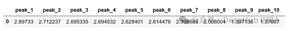
我们选择N = 10个峰值,但信号实际上只有M = 4个峰值,剩余的6个位置和峰值振幅将为0。

5、使用哪种方法?

我们已经看到了4种不同类别的方法。

我们应该使用哪一种?

如果你有一个基于领域的特征提取,那总是最好的选择:如果实验的物理或问题的先验知识是清晰的,你应该依赖于它并将这些特征视为最重要的,甚至可能将它们视为唯一的特征。

就频率、统计和基于时间的特征而言,在可以将它们一起使用。将这些特征添加到你的数据集中,然后看看其中的一些是否有帮助,没有帮助就把他们删除掉，这是一个测试的过程，就像超参数搜索一样，我们无法确定好坏，所以只能靠最后的结果来判断。

作者：Piero Paialunga

原创作者: deephub 转载于: https://blog.51cto.com/deephub/11899376