


模拟退火算法
* 注:该内容为个人收集总结其中也包含自己的一些理解,有点唠叨,就做个学习参考。
1.1、简介
模拟退火算法(Simulated Annealing,SA)思想由Metropolis等人于1953年提出并由Kirkpatrick等人于1983年引入到组合优化领域。SA算法模拟物理中固体加热后徐徐降温,内部能量逐渐趋于平衡状态的过程。其灵魂就是Metropolis准则,核心思想即以一定概率接受降温迭代过程中的较差解,以此在优化过程中更有利于跳出局部最优,逐渐逼近最优解。SA算法在理论上已经证明可以达全局最小值,研究现状包括SA算法的改进以及参数设置的研究;SA算法针对具体问题的应用研究等,并在机器学习、神经网络、图像识别、VLSI设计等领域有广泛的应用。
整体框架:
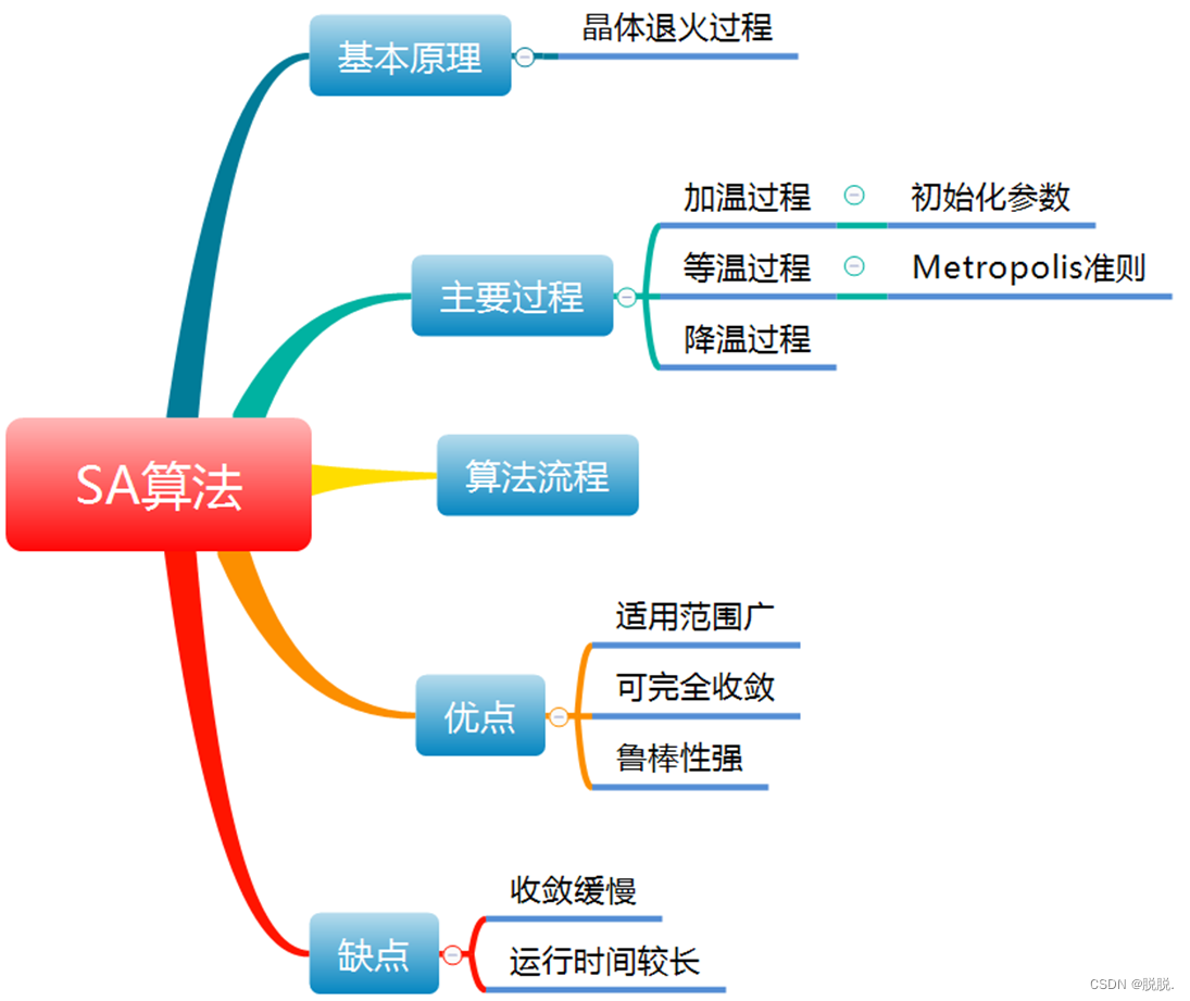
1.2、模拟退火算法的基本原理
退火即晶体冷却的过程,将一个物体加热至一定温度以后,釜底抽薪使其温度逐渐降到原来状态。在物理中,内能越高的物体,内部粒子随机运动越剧烈,此时物体状态十分不稳定,粒子的运动会随着温度的降低逐渐变得缓慢,当温度降低速度足够缓慢的时候,以原子晶体为例,其内部原子就有足够的时间排列成原来的结构模样,此时晶体内能最小达到稳定状态,这可以理解为是最优解;相反,当温度降低过快时,原子没有足够的时间排列成原有的结构,形成了能量较高的非晶体,这可以看成是局部最优解。
以上是退火物理过程,模拟退火算法就是在这个基础上诞生的,早期运用于解决组合优化问题中,模拟退火算法有以下几个过程:
(1)加温过程:
给晶体加温,使晶体内能增大其内部粒子剧烈运动,当温度高到一定程度时晶体熔化原系统内可能存在的非均匀的状态。对应于算法中即设置初始温度,而内能类似于遗传算法中的适应度函数和蚁群算法的启发函数,对应于模拟退火算法中的代价函数。
(2)等温过程
在物理学中指的是热力学系统的始末温度恒定内能不变,即晶体在降温过程中存在这样一个平衡过程,释放给周围环境的热量与从周围环境吸收的热量一样导致过程中系统环境温度不变。这个过程对应于算法中一个关键性的操作即根据Metropolis准则筛选解。Metropolis准则是模拟退火算法的灵魂,即算法在选择较优解之外再以一定的概率接受较差的解,这是使模拟退火算法不容易陷入局部最优的关键,没有它模拟退火算法等同于爬山算法。
(3)降温过程
降温过程即晶体温度逐渐下降的过程,温度下降速度对晶体冷却效果的影响在上文已经阐述过,在算法中通过降温系数控制,降温系数一般取小于1的正数,直接影响算法执行时间的长短和优化效率。
1.3、模拟退火算法的基本流程
模拟退火算法与遗传算法和蚁群算法一样,初始解都是随机生成,只不过前者是单体搜索算法,后者是群体搜索算法,模拟退火算法中新的解来源于上一个解,随机生成一个初始解后对这个解以一定的扰动策略产生新的解。通过Metropolis准则决定是接受新解还是旧解,在扰动和Metropolis准则判断过程中(等温过程),通常会使用蒙特卡洛方法对每一个温度下的等温过程给予一个蒙特卡洛循环迭代,这是为了在当前温度下找到一个更好的状态。蒙特卡洛循环是以大数定理作为理论基础,实验重复次数越多即所选的样本数量越多,其平均值就越接近真实结果。
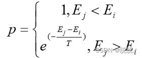
1.3.1、Metropolis准则
从当前状态i到新状态j,能量分别为 和
和 ,则接受新状态的概率p为:
以最小化问题为例描述模拟退化算法大致过程:
(1)初始化算法参数:随机生成初始解即当前解 ,设置合适的初始温度
 ,且当前温度
 ,设置蒙特卡洛循环次数;
(2)对当前解 以一定的扰动策略生成一个新解
 ;
;
(3) 计算两个解之间的能量差值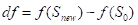 ;
; 是
是 的代价函数;若
 说明新解更优,以1的概率直接接受新解即
 ;若df>0;即当前解更优,但仍以
 的概率接受
的概率接受 ,在**[0,1]**之间生成一个伪随机数
 ,若
,若 ,则接受该新解
 ;否则
;否则 ;
;
(4)对(2)(3)(4)步执行一定次数的蒙特卡洛循环。
(5)更新当前温度,判断是否满足算法停止条件,若是则停止算法输出解 ,否则返回步骤(2)继续执行。
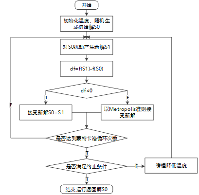
1.3.2、流程图
模拟退火算法的流程如图2-6所示:
1.4、 模拟退火算法的特点
(1) 模拟搜索算法是单体搜索算法,算法流程简单明了,通用性强,鲁棒性强,多应用于组合优化问题和非线性优化问题等。
(2) 模拟退火算法通常运行时间略长,因为其算法的特性,初始温度设置一般较高,降温系数较小,才能更有效地收敛到最优解,再加上内部有蒙特卡洛循环,使得算法运行时间较遗传和蚁群算法来讲较长。
(3) 模拟退火算法是被证明的可以完全收敛到最优解的算法,但收敛速度较缓慢,因为Metropolis准则的原因,有一部分解是接受的较差解,所以并不是全程都在收敛中。
2.1、模拟退火算法处理TSP问题
组合优化问题,TSP问题见遗传算法(GA)分析总结
根据上文描述的模拟退火算法的思想,对处理TSP问题作以下几点设置:
(1) 初始解为随机生成的1-n的整数;
(2) 扰动策略选择随机两个城市序号互换;
(3) 代价函数选择路径总长度的计算函数;
(4) 停止条件选择温度降到一定数值停止。
使用Matlab语言实现,参数设置如下:
停止温度:0.001;降温系数:0.99;蒙特卡洛循环次数:100;城市数据:att48.txt;初始温度分别取:1000、2400、4800(城市数量*100作为初始温度,迭代1531次);不同初始温度分别运行5次后取最短路径长度,所得数据结果如表所示(注:括号内为收敛于第多少代):
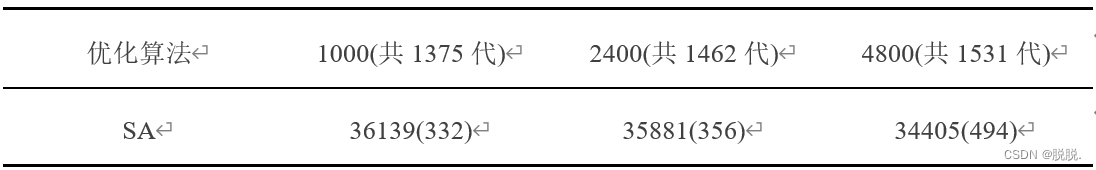
最优结果路线及收敛信息如图3-3所示:

该参数下的模拟退火算法最久会在运行500代内会收敛。
结果数据分析见遗传算法(GA)分析总结3.1.1
优化质量分析见遗传算法(GA)分析总结3.1.2
收敛性分析见遗传算法(GA)分析总结3.1.3
2.2、Matlab代码模拟处理TSP
main.m(注释的代码可忽略)
clear all;
close all;
clc
tic
C=[3245.00 3305.00;
        3484.00 2829.00;
        3023.00 1942.00;
        3082.00 1644.00;
        1916.00 1569.00;
        1633.00 2809.00;
        1112.00 2049.00;
        10.00 2676.00;
        23.00 2216.00;
        401.00 841.00;
        675.00 1006.00;
        2233.00 10.00;
        3177.00 756.00;
        4608.00 1198.00;
        4985.00 140.00;
        6107.00 669.00;
        6101.00 1110.00;
        5530.00 1424.00;
        5199.00 2182.00;
        4612.00 2035.00;
        4307.00 2322.00;
        4706.00 2674.00;
        5468.00 2606.00;
        5989.00 2873.00;
        6347.00 2683.00;
        6271.00 2135.00;
        6898.00 1885.00;
        6734.00 1453.00;
        7265.00 1268.00;
        7392.00 2244.00;
        7545.00 2801.00;
        7509.00 3239.00;
        7462.00 3590.00;
        7573.00 3716.00;
        7541.00 3981.00;
        7608.00 4458.00;
        7762.00 4595.00;
        7732.00 4723.00;
        7555.00 4819.00;
        7611.00 5184.00;
        7280.00 4899.00;
        7352.00 4506.00;
        7248.00 3779.00;
        6807.00 2993.00;
        6426.00 3173.00;
        5900.00 3561.00;
        5185.00 3258.00;
        4483.00 3369.00;
];
[cityNum,~] = size(C);        %城市个数
% 求任意两个城市之间的距离
for m=1:cityNum
    for n=1:cityNum
        distance(m,n) = sqrt(sum((C(m,:)-C(n,:)).^2));
    end
end
iter=100;        %内部蒙特卡洛循环迭代次数
% T=iter*cityNum;        %初始温度
T=2400
T_stop = 0.001;  %停止温度
T_decline = 0.99 %温度下降系数
%计算迭代次数
Time = ceil(log((T_stop)/T)/log(T_decline));
L_best = inf.*ones(Time+1,1);
S = randperm(cityNum); %产生一个随机解
t=1;                            %统计迭代次数
L_best(t)=CalRouteLength(distance,S);   %每次迭代后的路线长度
%netplot(city,n);               %初始旅行路线(做对比)
acceptTime=0;
gen = 0;
while T>=T_stop       %停止迭代温度
    for i=1:iter     %多次迭代扰动,蒙特卡洛方法,温度降低之前多次实验
        len1=CalRouteLength(distance,S);         %计算原路线总距离
        tmp_city=perturb(S,cityNum);      %产生随机扰动
        len2=CalRouteLength(distance,tmp_city);     %计算新路线总距离

        delta_e=len2-len1;  %新老距离的差值,相当于能量
        if delta_e<0        %新路线好于旧路线,用新路线代替旧路线
            S=tmp_city;
        else                        %温度越低,越不太可能接受新解;新老距离差值越大,越不太可能接受新解
            acceptProb = exp(-delta_e/T);
            r = rand();
            if acceptProb>r %以概率选择是否接受新解
                S=tmp_city;      %可能得到较差的解
                acceptTime = acceptTime+1;
            end
        end
    end
    t=t+1;
    L_best(t)=CalRouteLength(distance,S);   %计算新路线距离
    T=T*T_decline;   %温度不断下降

%     一边运行一边显示结果,速度更慢
%     figure(1);
%     for i=1:n-1
%         plot([C(S(i),1) C(S(i+1),1)],[C(S(i),2) C(S(i+1),2)],'bo-'); %只连线当前城市和下家城市
%         hold on;
%     end
%     plot([C(S(n),1) C(S(1),1)],[C(S(n),2) C(S(1),2)],'ro-'); %最后一家城市连线第一家城市
%     xlabel('城市位置横坐标')
%     ylabel('城市位置纵坐标')
%     title(['迭代次数:',int2str(gen),' 优化最短距离:',num2str(min(L_best))]);
%     hold off;
%     pause(0.001);
%
%     figure(2);
%     plot(L_best);
%     title('路径长度变化曲线');
%     xlabel('迭代次数');
%     ylabel('路径长度数值');

    gen=gen+1;
end
%只显示最后的结果,速度更快
figure;
netplot(S,cityNum,C,gen,L_best);    %最终旅行路线
%收敛情况
figure;
plot(L_best);
title('路径长度变化曲线');
xlabel('迭代次数');
ylabel('路径长度数值');
disp(L_best(end));
toc
CalRouteLength.m
% 计算一条染色体的适应度
% chromo 为一条染色体,即一条路径
function S_Value = CalRouteLength(distances, S)
RouteLength = 0;
n = size(S, 2); % 染色体的长度
for i = 1 : (n - 1)
    RouteLength = RouteLength + distances(S(i), S(i + 1));
end
RouteLength = RouteLength + distances(S(n), S(1));
S_Value = RouteLength;
end
netplot.m
function netplot(city,n,C,gen,L_best)        %连线各城市,将路线画出来
    hold on;
    for i=1:n-1
        plot([C(city(i),1) C(city(i+1),1)],[C(city(i),2) C(city(i+1),2)],'bo-'); %只连线当前城市和下家城市
        xlabel('城市位置横坐标')
        ylabel('城市位置纵坐标')
    end
    plot([C(city(n),1) C(city(1),1)],[C(city(n),2) C(city(1),2)],'ro-'); %最后一家城市连线第一家城市
    title(['迭代次数:',int2str(gen),' 优化最短距离:',num2str(min(L_best))]);
    hold off;
end
perturb.m
function S1=perturb(S,n)

    %随机置换两个不同的城市的坐标
    %产生随机扰动
    S1(1,:)=S(1,:);
    p1=floor(1+n*rand());
    p2=floor(1+n*rand());
    while p1==p2
        p1=floor(1+n*rand());
        p2=floor(1+n*rand());
    end
    %tmp=S(p1);
    S1(p1)=S(p2);
    S1(p2)=S(p1);
end
3.1、C#模拟
SA算法处理TSP问题实验界面如图:
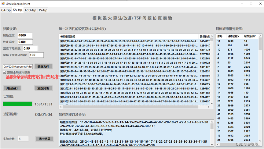
界面控件功能参考遗传算法(GA)分析总结里遗传算法仿真实验界面。
SA算法结果显示上只设置了最基本的结果信息。开发环境使用Visual Studio 2019(vs2019)、开发语言C#以及.NET Framework Windows窗体应用开发类库。
VS项目文件链接,有需要的可以作学习参考:C#仿真程序资源


 477
477


 被折叠的 条评论
为什么被折叠?
被折叠的 条评论
为什么被折叠?
 到【灌水乐园】发言


