365打卡第R6周: LSTM实现糖尿病探索与预测-CSDN博客

本文链接：https://blog.csdn.net/weixin_42570076/article/details/147683996

🍨 本文为🔗365天深度学习训练营中的学习记录博客
🍖 原作者：K同学啊

🏡 我的环境：

语言环境：Python3.10
编译器：Jupyter Lab
深度学习环境：torch==2.5.1 torchvision==0.20.1
------------------------------分割线---------------------------------

#设置GPU 
import torch.nn as nn 
import torch.nn.functional as F 
import torchvision,torch 
 
device = torch.device("cuda" if torch.cuda.is_available() else "cpu")
 
print(device)

(数据规模很小，在普通笔记本电脑就可以流畅跑完)

#导入数据
import numpy   as np
import pandas  as pd
import seaborn as sns
from sklearn.model_selection import train_test_split
import matplotlib.pyplot as plt
plt.rcParams['savefig.dpi'] = 500 #图片像素
plt.rcParams['figure.dpi'] = 500 #分辨率
 
plt.rcParams['font.sans-serif'] = ['SimHei'] #用来正常显示中文标签
 
import warnings
warnings.filterwarnings('ignore')
 
DataFrame = pd.read_excel('./dia.xls')
print(DataFrame.head())
 
print(DataFrame.shape)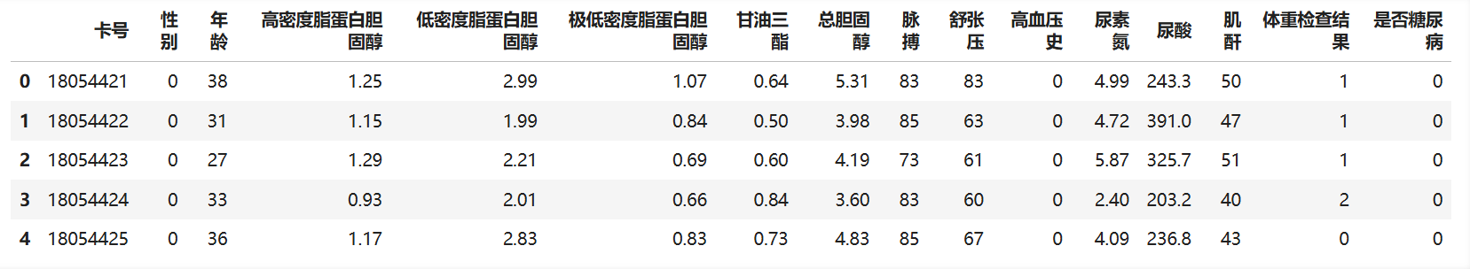

# 查看是否有缺失值
print("数据缺失值------------------")
print(DataFrame.isnull().sum())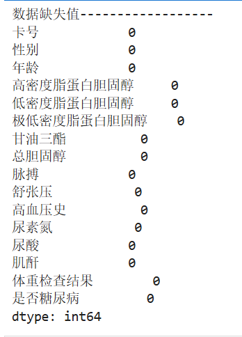

# 查看数据是否有重复值
print("数据重复值------------------")
print('数据的重复值为：'f'{DataFrame.duplicated().sum()}')

feature_map = {
            '年龄': '年龄',
            '高密度脂蛋白胆固醇': '高密度脂蛋白胆固醇',
            '低密度脂蛋白胆固醇': '低密度脂蛋白胆固醇',
            '极低密度脂蛋白胆固醇': '极低密度脂蛋白胆固醇',
            '甘油三酯': '甘油三酯',
            '总胆固醇': '总胆固醇',
            '脉搏': '脉搏',
            '舒张压': '舒张压',
            '高血压史': '高血压史',
            '尿素氮': '尿素氮',
            '尿酸': '尿酸',
            '肌酐': '肌酐',
            '体重检查结果': '体重检查结果'
}
 
plt.figure(figsize=(15, 10))
for i, (col, col_name) in enumerate(feature_map.items(), 1):
    plt.subplot(3, 5, i)
    sns.boxplot(x=DataFrame['是否糖尿病'], y=DataFrame[col])
    plt.title(f'{col_name}的箱线图', fontsize=14)
    plt.ylabel('数值', fontsize=12)
    plt.grid(axis='y', linestyle='--', alpha=0.7)
plt.tight_layout()
plt.show()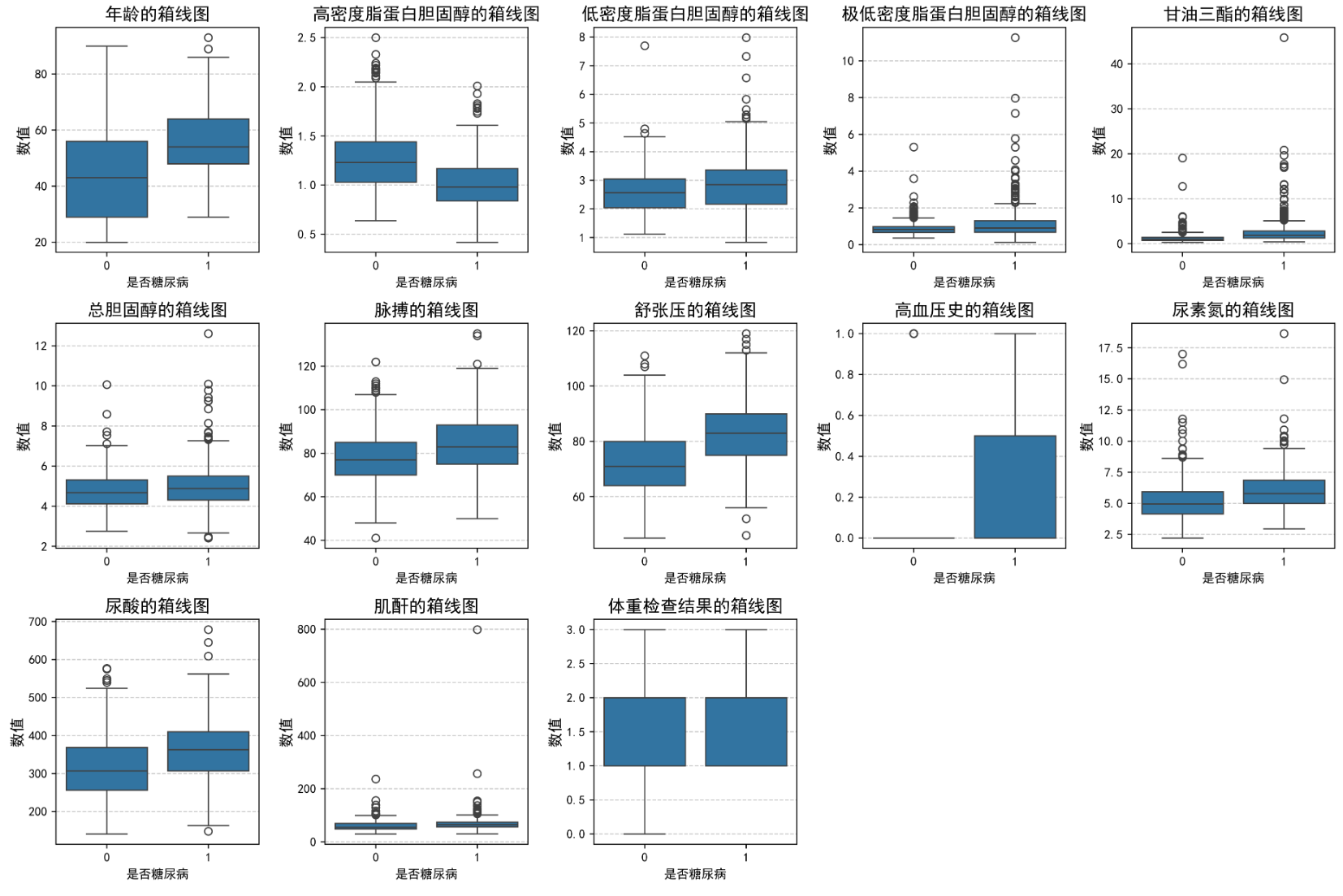

# 构建数据集
from sklearn.preprocessing import StandardScaler
 
# '高密度脂蛋白胆固醇'字段与糖尿病负相关，故在X 中去掉该字段
X = DataFrame.drop(['卡号', '是否糖尿病', '高密度脂蛋白胆固醇'], axis=1)
y = DataFrame['是否糖尿病']
 
# sc_X = StandardScaler()
# X = sc_X.fit_transform
 
X = torch.tensor(np.array(X), dtype=torch.float32)
y = torch.tensor(np.array(y), dtype=torch.int64)
 
train_X, test_X, train_y, test_y = train_test_split(X, y, test_size=0.2, random_state=1)
 
train_X.shape, train_y.shape

from torch.utils.data import TensorDataset, DataLoader
 
train_dl = DataLoader(TensorDataset(train_X, train_y), 
                      batch_size=64, 
                      shuffle=False)
test_dl = DataLoader(TensorDataset(test_X, test_y), 
                      batch_size=64, 
                      shuffle=False)

# 定义模型
class model_lstm(nn.Module):
    def __init__(self):
        super(model_lstm, self).__init__()
 
        self.lstm0 = nn.LSTM(input_size=13, hidden_size=200,
                             num_layers=1, batch_first=True)
 
        self.lstm1 = nn.LSTM(input_size=200, hidden_size=200,
                             num_layers=1, batch_first=True)
        self.fc0 = nn.Linear(200, 2)  # 输出 2 类
 
    def forward(self, x):
        # 如果 x 是 2D 的，转换为 3D 张量，假设 seq_len=1
        if x.dim() == 2:
            x = x.unsqueeze(1)  # [batch_size, 1, input_size]
        
        # LSTM 处理数据
        out, (h_n, c_n) = self.lstm0(x)  # 第一层 LSTM
        
        # 使用第二个 LSTM，并传递隐藏状态
        out, (h_n, c_n) = self.lstm1(out, (h_n, c_n))  # 第二层 LSTM
        
        # 获取最后一个时间步的输出
        out = out[:, -1, :]  # 选择序列的最后一个时间步的输出
        
        out = self.fc0(out)  # [batch_size, 2]
        return out
 
model = model_lstm().to(device)
print(model)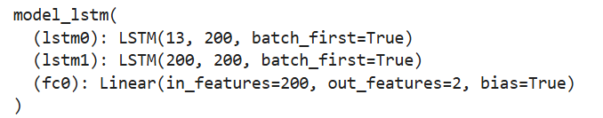

# 训练模型

def train(dataloader, model, loss_fn, optimizer):
    size = len(dataloader.dataset)  # 训练集的大小
    num_batches = len(dataloader)  # 批次数目
    train_loss, train_acc = 0, 0  # 初始化训练损失和正确率
 
    model.train()  # 设置模型为训练模式
    for X, y in dataloader:  # 获取数据和标签
        
        # 如果 X 是 2D 的，调整为 3D
        if X.dim() == 2:
            X = X.unsqueeze(1)  # [batch_size, 1, input_size]，即假设 seq_len=1
        
        X, y = X.to(device), y.to(device)  # 将数据移动到设备
 
        # 计算预测误差
        pred = model(X)  # 网络输出
        loss = loss_fn(pred, y)  # 计算网络输出和真实值之间的差距
 
        # 反向传播
        optimizer.zero_grad()  # 清除上一步的梯度
        loss.backward()  # 反向传播
        optimizer.step()  # 更新权重
 
        # 记录acc与loss
        train_acc += (pred.argmax(1) == y).type(torch.float).sum().item()
        train_loss += loss.item()
 
    train_acc /= size  # 平均准确率
    train_loss /= num_batches  # 平均损失
    return train_acc, train_loss

def test(dataloader, model, loss_fn):
    size = len(dataloader.dataset)  # 测试集的大小
    num_batches = len(dataloader)  # 批次数目, (size/batch_size，向上取
    test_loss, test_acc = 0, 0
 
    # 当不进行训练时，停止梯度更新，节省计算内存消耗
    with torch.no_grad():
        for imgs, target in dataloader:
            imgs, target = imgs.to(device), target.to(device)
 
            # 计算loss
            target_pred = model(imgs)
            loss = loss_fn(target_pred, target)
 
            test_loss += loss.item()
            test_acc += (target_pred.argmax(1) == target).type(torch.float).sum().item()
    test_acc /= size
    test_loss /= num_batches
    return test_acc, test_loss

loss_fn = nn.CrossEntropyLoss()  # 创建损失函数
learn_rate = 1e-4  # 学习率
opt = torch.optim.Adam(model.parameters(), lr=learn_rate)
epochs = 50
train_loss = []
train_acc = []
test_loss = []
test_acc = []
for epoch in range(epochs):
    model.train()
    epoch_train_acc, epoch_train_loss = train(train_dl, model, loss_fn, opt)
    model.eval()
    epoch_test_acc, epoch_test_loss = test(test_dl, model, loss_fn)
    train_acc.append(epoch_train_acc)
    train_loss.append(epoch_train_loss)
    test_acc.append(epoch_test_acc)
    test_loss.append(epoch_test_loss)
 
    # 获取当前的学习率
    lr = opt.state_dict()['param_groups'][0]['lr']
 
    template = ('Epoch:{:2d}, Train_acc:{:.1f}%, Train_loss:{:.3f}, Test_acc:{:.1f}%, Test_loss:{:.3f},Lr:{:.2E}')
    print(
        template.format(epoch + 1, epoch_train_acc * 100, epoch_train_loss, epoch_test_acc * 100, epoch_test_loss, lr))
 
print("=" * 20, 'Done', "=" * 20)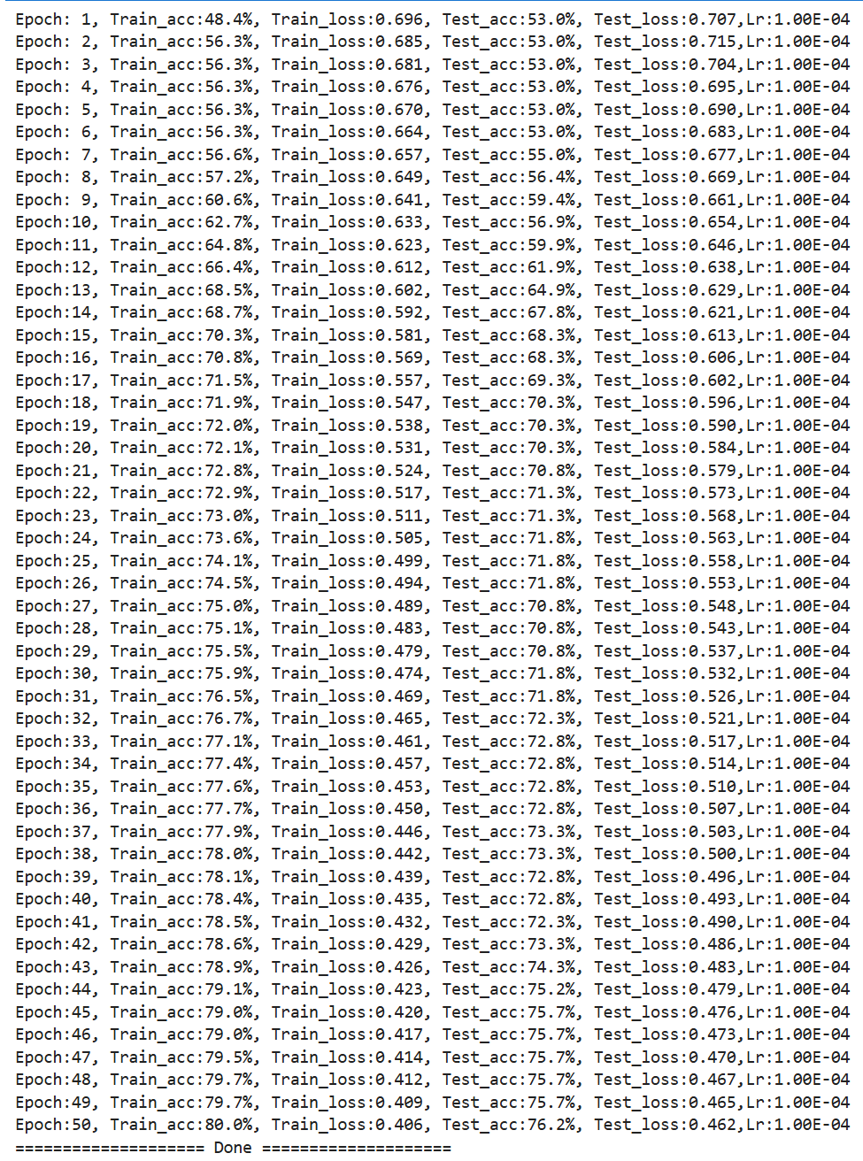

import matplotlib.pyplot as plt
#隐藏警告
import warnings
warnings.filterwarnings("ignore")               #忽略警告信息
plt.rcParams['font.sans-serif']    = ['SimHei'] # 用来正常显示中文标签
plt.rcParams['axes.unicode_minus'] = False      # 用来正常显示负号
plt.rcParams['figure.dpi']         = 100        #分辨率
 
from datetime import datetime
current_time = datetime.now()
 
epochs_range = range(epochs)
 
plt.figure(figsize=(12, 3))
plt.subplot(1, 2, 1)
 
plt.plot(epochs_range, train_acc, label='Training Accuracy')
plt.plot(epochs_range, test_acc, label='Test Accuracy')
plt.legend(loc='lower right')
plt.title('Training and Validation Accuracy')
plt.xlabel(current_time)
 
plt.subplot(1, 2, 2)
plt.plot(epochs_range, train_loss, label='Training Loss')
plt.plot(epochs_range, test_loss, label='Test Loss')
plt.legend(loc='upper right')
plt.title('Training and Validation Loss')
plt.show()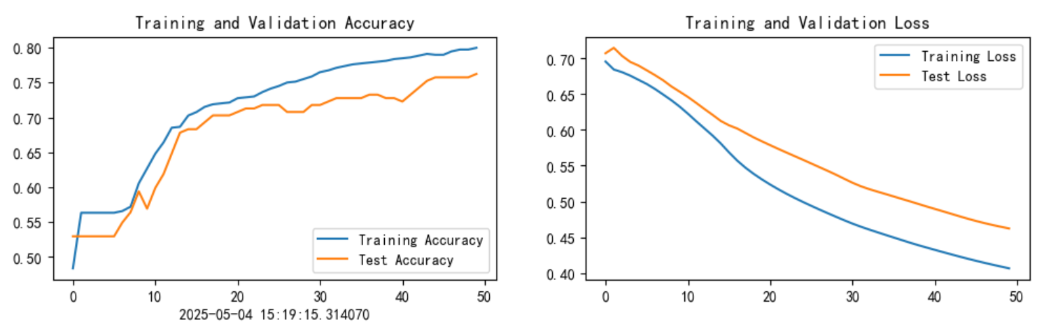

--------------小结和改进思路（顺便把R7周的任务一起完成）---------------------

针对前述代码，主要在下面几个方面进行改进：

性能提升：通过双向LSTM和Dropout增强特征提取能力，标准化和类别权重缓解数据问题。
防止过拟合：在全连接层前添加BatchNorm提高泛化性。
训练稳定性：学习率调度器和训练集启用shuffle随机打乱数据使训练更稳定。

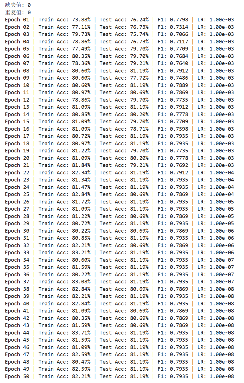
通过上述优化，模型在保持LSTM核心结构的同时，能够更有效地处理表格数据并提升预测性能，最终训练集和测试集分别提高了5个百分点。

import torch
import torch.nn as nn
import torch.optim as optim
from torch.utils.data import TensorDataset, DataLoader
import numpy as np
import pandas as pd
from sklearn.model_selection import train_test_split
from sklearn.preprocessing import StandardScaler
from sklearn.metrics import f1_score, confusion_matrix
import matplotlib.pyplot as plt
import seaborn as sns

# 环境设置
device = torch.device("cuda" if torch.cuda.is_available() else "cpu")
device

plt.rcParams['font.sans-serif'] = ['SimHei']
plt.rcParams['axes.unicode_minus'] = False
torch.manual_seed(42) # 打印随机seed使随机分配可重复

# 数据加载与预处理
def load_data():
    df = pd.read_excel('./dia.xls')
    
    # 数据清洗
    print("缺失值:", df.isnull().sum().sum())
    print("重复值:", df.duplicated().sum())
    df = df.drop_duplicates().reset_index(drop=True)
    
    # 特征工程
    X = df.drop(['卡号', '是否糖尿病', '高密度脂蛋白胆固醇'], axis=1)
    y = df['是否糖尿病']
    
    # 处理类别不平衡
    class_counts = y.value_counts().values
    class_weights = torch.tensor([1/count for count in class_counts], dtype=torch.float32).to(device)
    
    # 数据标准化（先分割后标准化）
    X_train, X_test, y_train, y_test = train_test_split(X, y, test_size=0.2, stratify=y, random_state=42)
    scaler = StandardScaler()
    X_train = scaler.fit_transform(X_train)
    X_test = scaler.transform(X_test)
    
    # 转换为Tensor
    X_train = torch.tensor(X_train, dtype=torch.float32).to(device)
    X_test = torch.tensor(X_test, dtype=torch.float32).to(device)
    y_train = torch.tensor(y_train.values, dtype=torch.long).to(device)
    y_test = torch.tensor(y_test.values, dtype=torch.long).to(device)
    
    return X_train, X_test, y_train, y_test, class_weights

# 双向LSTM模型
class BiLSTM(nn.Module):
    def __init__(self, input_size=12, hidden_size=100, num_layers=2):
        super().__init__()
        self.lstm = nn.LSTM(
            input_size=input_size,
            hidden_size=hidden_size,
            num_layers=num_layers,
            bidirectional=True,
            batch_first=True,
            dropout=0.3 if num_layers>1 else 0
        )
        self.bn = nn.BatchNorm1d(hidden_size*2)
        self.dropout = nn.Dropout(0.5)
        self.fc = nn.Linear(hidden_size*2, 2)
        
    def forward(self, x):
        if x.dim() == 2:
            x = x.unsqueeze(1)
        out, _ = self.lstm(x)
        out = out[:, -1, :]  # 取最后时间步
        out = self.bn(out)
        out = self.dropout(out)
        return self.fc(out)

# 训练与验证函数
def train_epoch(model, loader, criterion, optimizer):
    model.train()
    total_loss, correct = 0, 0
    
    for X, y in loader:
        X = X.unsqueeze(1) if X.dim()==2 else X
        optimizer.zero_grad()
        outputs = model(X)
        loss = criterion(outputs, y)
        loss.backward()
        optimizer.step()
        
        total_loss += loss.item()
        correct += (outputs.argmax(1) == y).sum().item()
        
    return correct/len(loader.dataset), total_loss/len(loader)

def evaluate(model, loader, criterion):
    model.eval()
    total_loss, correct = 0, 0
    all_preds, all_labels = [], []
    
    with torch.no_grad():
        for X, y in loader:
            X = X.unsqueeze(1) if X.dim()==2 else X
            outputs = model(X)
            loss = criterion(outputs, y)
            
            total_loss += loss.item()
            correct += (outputs.argmax(1) == y).sum().item()
            all_preds.extend(outputs.argmax(1).cpu().numpy())
            all_labels.extend(y.cpu().numpy())
    
    f1 = f1_score(all_labels, all_preds)
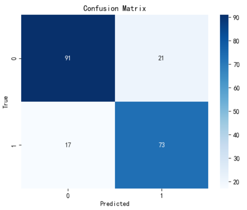
    cm = confusion_matrix(all_labels, all_preds)
    return correct/len(loader.dataset), total_loss/len(loader), f1, cm

print(model)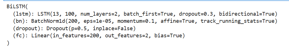


    # 数据准备
    X_train, X_test, y_train, y_test, class_weights = load_data()
    
    train_dataset = TensorDataset(X_train, y_train)
    test_dataset = TensorDataset(X_test, y_test)
    
    train_loader = DataLoader(train_dataset, batch_size=64, shuffle=True)
    test_loader = DataLoader(test_dataset, batch_size=64)
    
    # 模型初始化
    model = BiLSTM(input_size=13).to(device)
    criterion = nn.CrossEntropyLoss(weight=class_weights)
    optimizer = optim.Adam(model.parameters(), lr=1e-3, weight_decay=1e-4)
    scheduler = optim.lr_scheduler.ReduceLROnPlateau(optimizer, 'min', patience=3)
    
    # 训练循环
    best_f1 = 0
    train_losses, test_losses = [], []
    train_accs, test_accs = [], []
    
    for epoch in range(50):
        train_acc, train_loss = train_epoch(model, train_loader, criterion, optimizer)
        test_acc, test_loss, f1, cm = evaluate(model, test_loader, criterion)
        
        # 学习率调整
        scheduler.step(test_loss)
        
        # 记录指标
        train_losses.append(train_loss)
        test_losses.append(test_loss)
        train_accs.append(train_acc)
        test_accs.append(test_acc)
              
        # 打印信息
        print(f"Epoch {epoch+1:02d} | "
              f"Train Acc: {train_acc:.2%} | Test Acc: {test_acc:.2%} | "
              f"F1: {f1:.4f} | LR: {optimizer.param_groups[0]['lr']:.2e}")
    
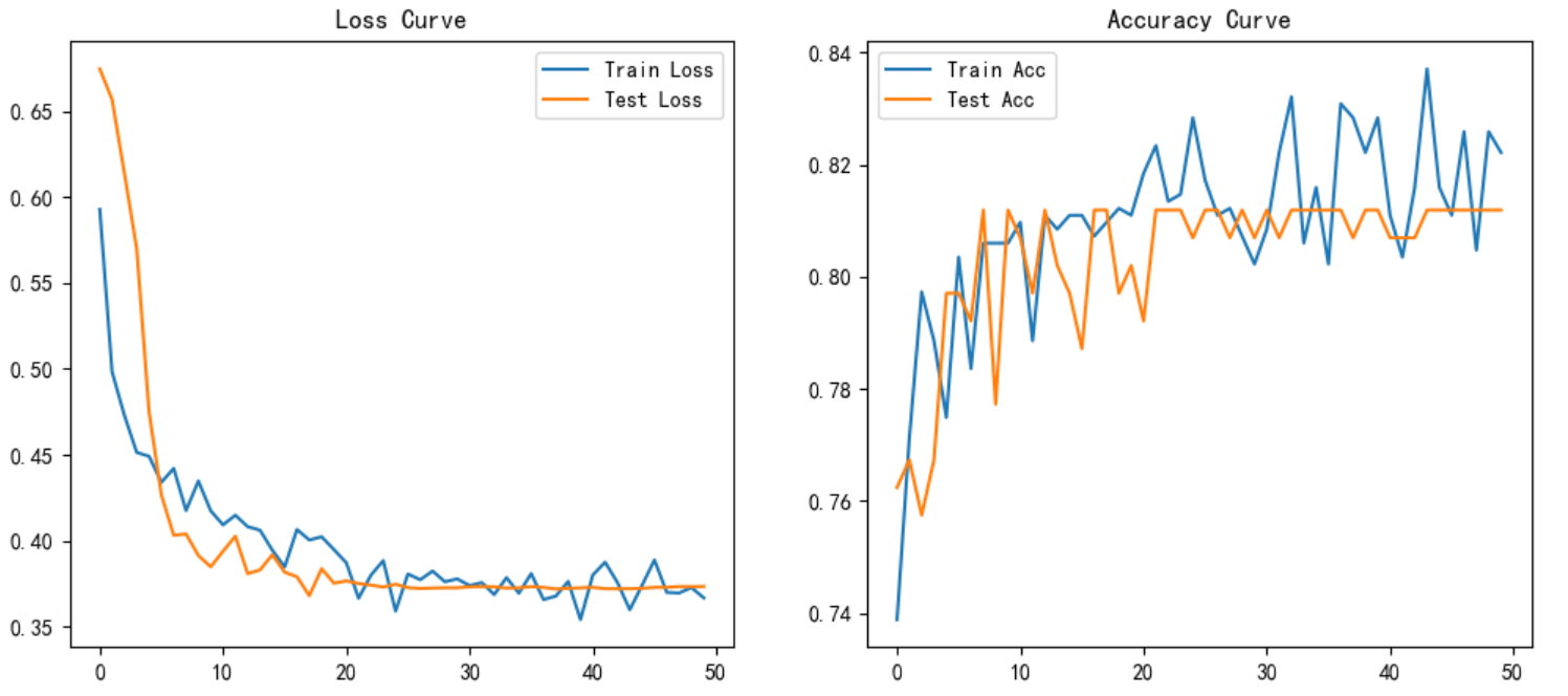
    # 可视化
    plt.figure(figsize=(12,5))
    plt.subplot(1,2,1)
    plt.plot(train_losses, label='Train Loss')
    plt.plot(test_losses, label='Test Loss')
    plt.legend()
    plt.title("Loss Curve")
    
    plt.subplot(1,2,2)
    plt.plot(train_accs, label='Train Acc')
    plt.plot(test_accs, label='Test Acc')
    plt.legend()
    plt.title("Accuracy Curve")
    plt.show()