opencv学习笔记

---

一、opencv入门

1.读取图像

import cv2
img = cv2.imread(filename[,flag])
# img是返回值，其值是读到的图像。如果未读到图像，则返回“None”
# filename是图像的完整的文件名，flag是读取标记

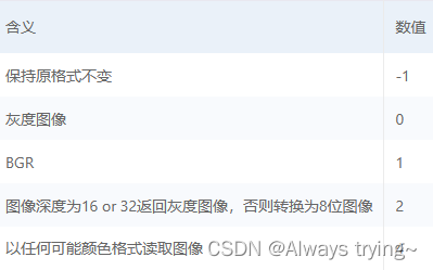
读取标记解释如下图：

2.展示图像

from PIL import Image
import numpy as np
import matplotlib.pylab as pylab
pylab.imshow(img)

3.保存图像

img=cv2.imwrite(filename,img[,params])
# img返回值，保存成功返回True，否则返回False
# filename是要保存的图像的完成路径名，包括扩展名

二、图像处理基础

1.二值图像

二值图像是指黑白图像，将图像上的像素点的灰度值设置为0或255.图像的二值化使得图像中数据量大为减少，从而能凸显出目标的轮廓。 要得到二值化图像，首先要把图像灰度化，然后将256个亮度等级的灰度图像通过选取适当的阈值来获得可以反映图像整体和局部特征的二值化图像

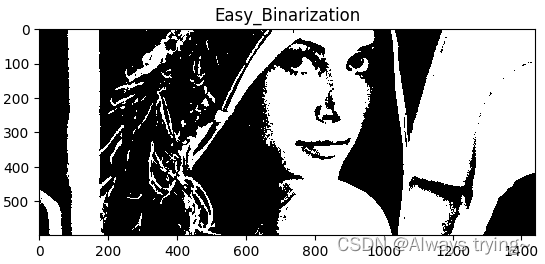
1.简单二值法

将图像灰度化后，将像素值大于127的像素值都设为255(纯白色)，小于127的都设为0(黑色)

import cv2
import matplotlib.pylab as plt
def Easy_Binarization(srcImg_path):
    img = cv2.imread(srcImg_path)
    img_gray = cv2.cvtColor(img, cv2.COLOR_BGR2GRAY)
    img_gray[img_gray>127] = 255
    img_gray[img_gray<=127] = 0
    plt.imshow(img_gray, cmap='gray')
    plt.title('Easy_Binarization')
    plt.show()
Easy_Binarization('例.jpg')

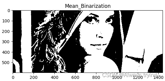
2.平均值法

为了应对每张图片的灰度值大不相同，阈值取为图像本身的平均值。

import cv2
import matplotlib.pylab as plt
def Mean_Binarization(srcImg_path):
    img = cv2.imread(srcImg_path)
    img_gray = cv2.cvtColor(img, cv2.COLOR_BGR2GRAY)
    threshold = np.mean(img_gray)
    print(threshold)
    img_gray[img_gray>threshold] = 255
    img_gray[img_gray<=threshold] = 0
    plt.imshow(img_gray, cmap='gray')
    plt.title('Mean_Binarization')
    plt.show()
Mean_Binarization('例.jpg')

3.双峰法

直方图是图像的重要特质，它可以帮助我们分析图像中的灰度变化。因此，如果物体与背景的灰度值对比明显，直方图就会包含双峰，它们分别为图像的前景和背景，而它们之间的谷底即为边缘附近相对较少数目的像素点，一般来讲，这个最小值就为最优二值化的分界点，通过这个点可以把前景和背景很好地分开。

import cv2
import matplotlib.pylab as plt
from collections import Counter
def Hist_Binarization(srcImg_path):
    img = cv2.imread(srcImg_path)
    img_gray = cv2.cvtColor(img, cv2.COLOR_BGR2GRAY)
    hist = img_gray.flatten()
    plt.subplot(121)
    plt.hist(hist,256)

    cnt_hist = Counter(hist)
    print(cnt_hist)
    begin,end = cnt_hist.most_common(2)[0][0],cnt_hist.most_common(2)[1][0]
    if begin > end:
        begin, end = end, begin
    print(f'{begin}: {end}')

    cnt = np.iinfo(np.int16).max
    threshold = 0
    for i in range(begin,end+1):
        if cnt_hist[i]<cnt:
            cnt = cnt_hist[i]
            threshold = i
    print(f'{threshold}: {cnt}')
    img_gray[img_gray>threshold] = 255
    img_gray[img_gray<=threshold] = 0
    plt.subplot(122)
    plt.imshow(img_gray, cmap='gray')
    plt.show()
Hist_Binarization('例.jpg')

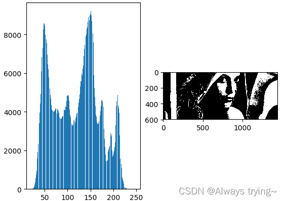
双峰法的缺点为直方图不连续，有很多的尖峰和抖动，要找到准确的极值点十分困难。

4.OTSU法

OTSU法也称作最大类间方差法，是按图像的灰度特性，将图像分成背景和前景两部分。因方差是灰度分布均匀性的一种度量,背景和前景之间的类间方差越大,说明构成图像的两部分的差别越大,当部分前景错分为背景或部分背景错分为前景都会导致类间差别变小。因此,使类间方差最大的分割意味着错分概率最小。

具体计算阈值方法如下：
设阈值为t, 将原图转化成灰度图后，将其高与宽存于h,w，并将小于阈值的灰度值存储在前景front中，大于等于阈值的存在背景back中。

def Otsu(srcImg_path):
    img = cv2.imread(srcImg_path)
    img = cv2.cvtColor(img, cv2.COLOR_BGR2GRAY)
    h, w = img.shape[:2]
    threshold_t = 0
    max_g = 0
 
    for t in range(255):
        front = img[img < t]
        back = img[img >= t]
        front_p = len(front) / (h * w)
        back_p = len(back) / (h * w)
        front_mean = np.mean(front) if len(front) > 0 else 0.
        back_mean = np.mean(back) if len(back) > 0 else 0.
        g = front_p * back_p * ((front_mean - back_mean)**2)
        if g > max_g:
            max_g = g
            threshold_t = t
    print(f"threshold = {threshold_t}")
    img[img < threshold_t] = 0
    img[img >= threshold_t] = 255
    plt.imshow(img, cmap='gray')
    plt.title('Otsu')
    plt.show()
Otsu('例.jpg')

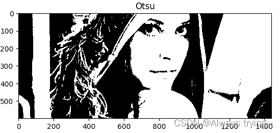
对比四种方法可得：Otsu方法得到的二值化图像细节更多，图像更细腻。

2.灰度图像

img = cv2.imread("./例.jpg")
img = cv2.cvtColor(img, cv2.COLOR_BGR2GRAY)	# 将BGR转为灰度
plt.imshow(img)

3.感兴趣区域(ROI)

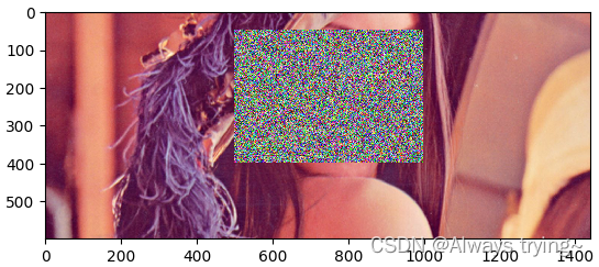
1.图像特定部分打码

a=cv2.imread("./例.jpg") #给lena面部打码
a[50:400,500:1000]=np.random.randint(0,256,(350,500,3))
a=cv2.cvtColor(a,cv2.COLOR_BGR2RGB) #将BGR转换成RGB
pylab.imshow(a)
cv2.imwrite("lena_面部打码.jpg",a)

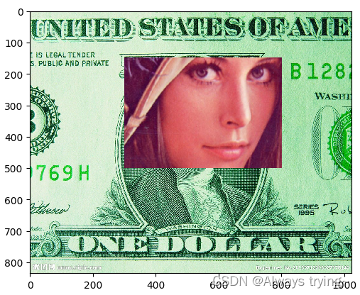
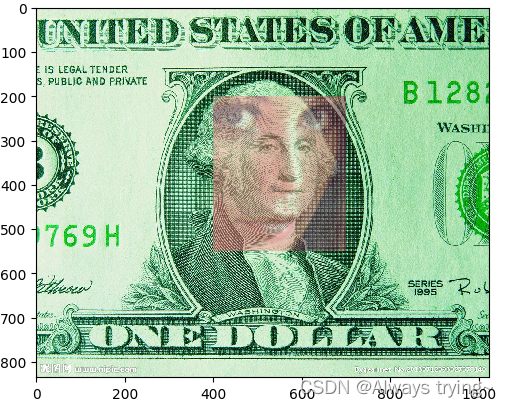
2.凸显图像特定部分

# 提取出面部区域
a=cv2.imread("./例.jpg") #提取lena的面部
face=a[50:400,500:1000]
face=cv2.cvtColor(face,cv2.COLOR_BGR2RGB) #将BGR转换成RGB
# 在另外一张图片上显示出面部区域
dollar=cv2.imread("./美元.jpg")
dollar=cv2.cvtColor(dollar,cv2.COLOR_BGR2RGB)
dollar[150:500,300:800]=face
pylab.imshow(dollar)
cv2.imwrite("dollar with dollar.jpg",dollar)

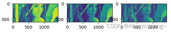
4.通道拆分

1.按索引拆分

from PIL import Image
import numpy as np
import matplotlib.pylab as pylab

lena=cv2.cvtColor(lena,cv2.COLOR_BGR2RGB) #将BGR转换成RGB
b=lena[:,:,0]
g=lena[:,:,1]
r=lena[:,:,2]
pylab.subplot(1,3,1)
pylab.imshow(b)
pylab.subplot(1,3,2)
pylab.imshow(g)
pylab.subplot(1,3,3)
pylab.imshow(r)

2.按函数拆分

b,g,r=cv2.split(lena)
pylab.subplot(1,3,1)
pylab.imshow(b)
pylab.subplot(1,3,2)
pylab.imshow(g)
pylab.subplot(1,3,3)
pylab.imshow(r)

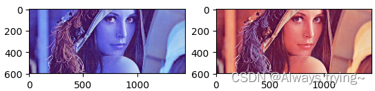
5.通道合并

lena=cv2.imread("例.jpg")
b,g,r=cv2.split(lena)# 将图像分为b,g,r三部分
bgr=cv2.merge([b,g,r]) #按照bgr顺序合并图像
rgb=cv2.merge([r,g,b]) #按照rgb顺序合并图像
pylab.subplot(1,2,1)
pylab.imshow(bgr)
pylab.subplot(1,2,2)
pylab.imshow(rgb)

三、图像运算

1.图像加权

在计算两幅图像的像素值之和时，将每幅图像的权重考虑进来，可以用公式表示为dst=saturate(src1×α+src×β+γ)

lena=cv2.imread("例.jpg")
lena=cv2.cvtColor(lena,cv2.COLOR_BGR2RGB)
dollar=cv2.imread("美元.jpg")
dollar=cv2.cvtColor(dollar,cv2.COLOR_BGR2RGB)
lena_face=lena[50:400,700:1000] #提取lena的脸
dollar_face=dollar[200:550,400:700] #提取美元的脸
result=cv2.addWeighted(lena_face,0.5,dollar_face,0.5,10) #对两张脸加权求和
dollar[200:550,400:700]=result
pylab.imshow(dollar)
cv2.imwrite("lena与dollar融合.jpg",dollar)

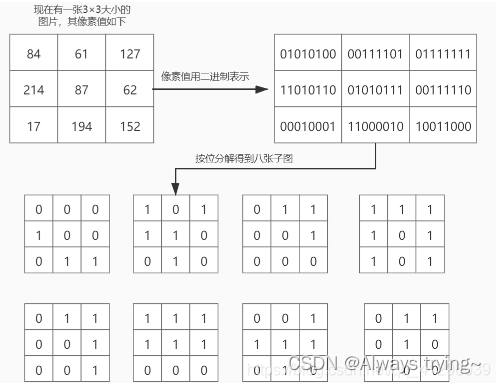
2.位平面分解

对于一般灰度图像而言，其灰度值通常是一个0到255之间的十进制数，那么每一个像素都可以由8位二进制序列唯一表示。因此，BBD可以将灰度图像拆分成8个二进制平面。第一个位平面是由灰度图像中每一个像素的二进制表示的所有第一位所组成的.