🌸 欢迎来到Python办公自动化专栏—Python处理办公问题,解放您的双手 📕 此外还有python基础专栏:请点击——>Python基础学习专栏 求订阅 文章作者技术和水平有限,如果文中出现错误,希望大家能指正🙏 ❤️ 欢迎各位佬关注! ❤️
Matplotlib 是 Python 中最流行的 2D 绘图库,用于创建高质量的静态、动态和交互式可视化。它最初由 John D. Hunter 于 2003 年创建,现已成为 Python 科学计算生态系统中的核心可视化工具。 主要特点
多功能性:支持线图、散点图、条形图、直方图、饼图、等高线图、3D 图等多种图表类型 高度可定制:几乎可以控制图形的每个元素(标题、标签、刻度、图例等) 多平台支持:可在多种操作系统和图形后端上工作 与其他库良好集成:与 NumPy、Pandas、SciPy 等科学计算库无缝协作 多种输出格式:支持 PNG、PDF、SVG、EPS 等多种格式输出 基本架构
Matplotlib 采用分层架构: Backend Layer:底层接口,处理不同输出格式和渲染 Artist Layer:中间层,处理图形元素(线、文本、图像等) Scripting Layer (pyplot):顶层接口,提供类似 MATLAB 的简单绘图命令 基本组件
Figure:整个图形窗口,可以包含多个子图 Axes:实际的绘图区域,包含坐标轴、标签等 Axis:坐标轴对象,控制刻度、标签等 Artist:所有可见元素(文本、线条、矩形等)的基类 Matplotlib的mplot3d工具包提供了多种3D数据可视化功能。下面介绍几种常见的3D图表类型及其实现方法。 库 用途 安装 numpy 数据生成 pip install numpy -i https://pypi.tuna.tsinghua.edu.cn/simple/matplotlib 数据可视化 pip install matplotlib -i https://pypi.tuna.tsinghua.edu.cn/simple/
import matplotlib. pyplot as plt
from mpl_toolkits. mplot3d import Axes3D
import numpy as np
from pylab import *
mpl. rcParams[ 'font.sans-serif' ] = [ 'SimHei' ]
mpl. rcParams[ 'axes.unicode_minus' ] = False
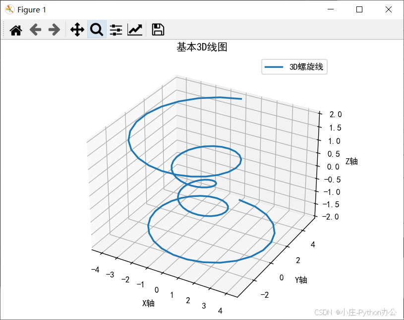
theta = np. linspace( - 4 * np. pi, 4 * np. pi, 100 )
z = np. linspace( - 2 , 2 , 100 )
r = z** 2 + 1
x = r * np. sin( theta)
y = r * np. cos( theta)
fig = plt. figure( figsize= ( 10 , 7 ) )
ax = fig. add_subplot( 111 , projection= '3d' )
ax. plot( x, y, z, label= '3D螺旋线' , linewidth= 2 )
ax. set_title( '基本3D线图' )
ax. set_xlabel( 'X轴' )
ax. set_ylabel( 'Y轴' )
ax. set_zlabel( 'Z轴' )
ax. legend( )
plt. tight_layout( )
plt. show( )
import matplotlib. pyplot as plt
from mpl_toolkits. mplot3d import Axes3D
import numpy as np
from pylab import *
mpl. rcParams[ 'font.sans-serif' ] = [ 'SimHei' ]
mpl. rcParams[ 'axes.unicode_minus' ] = False
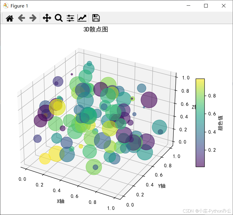
np. random. seed( 42 )
n = 100
x = np. random. rand( n)
y = np. random. rand( n)
z = np. random. rand( n)
colors = np. random. rand( n)
sizes = 1000 * np. random. rand( n)
fig = plt. figure( figsize= ( 10 , 7 ) )
ax = fig. add_subplot( 111 , projection= '3d' )
scatter = ax. scatter( x, y, z, c= colors, s= sizes, alpha= 0.6 , cmap= 'viridis' )
cbar = fig. colorbar( scatter, shrink= 0.5 , aspect= 10 )
cbar. set_label( '颜色值' )
ax. set_title( '3D散点图' )
ax. set_xlabel( 'X轴' )
ax. set_ylabel( 'Y轴' )
ax. set_zlabel( 'Z轴' )
plt. tight_layout( )
plt. show( )
import matplotlib. pyplot as plt
from mpl_toolkits. mplot3d import Axes3D
import numpy as np
from pylab import *
mpl. rcParams[ 'font.sans-serif' ] = [ 'SimHei' ]
mpl. rcParams[ 'axes.unicode_minus' ] = False
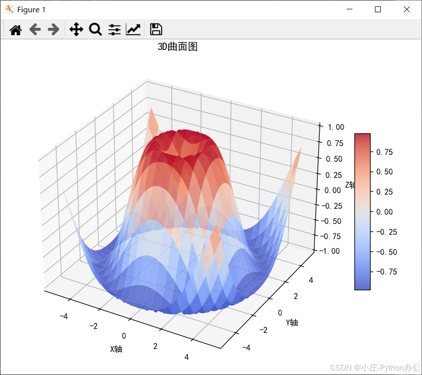
x = np. linspace( - 5 , 5 , 100 )
y = np. linspace( - 5 , 5 , 100 )
X, Y = np. meshgrid( x, y)
Z = np. sin( np. sqrt( X** 2 + Y** 2 ) )
fig = plt. figure( figsize= ( 12 , 8 ) )
ax = fig. add_subplot( 111 , projection= '3d' )
surf = ax. plot_surface( X, Y, Z, cmap= 'coolwarm' ,
linewidth= 0 , antialiased= True ,
rstride= 5 , cstride= 5 , alpha= 0.8 )
fig. colorbar( surf, shrink= 0.5 , aspect= 10 )
ax. set_title( '3D曲面图' )
ax. set_xlabel( 'X轴' )
ax. set_ylabel( 'Y轴' )
ax. set_zlabel( 'Z轴' )
plt. tight_layout( )
plt. show( )
import matplotlib. pyplot as plt
from mpl_toolkits. mplot3d import Axes3D
import numpy as np
from pylab import *
mpl. rcParams[ 'font.sans-serif' ] = [ 'SimHei' ]
mpl. rcParams[ 'axes.unicode_minus' ] = False
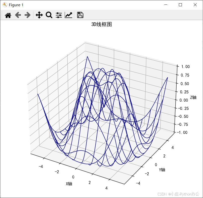
x = np. linspace( - 5 , 5 , 100 )
y = np. linspace( - 5 , 5 , 100 )
X, Y = np. meshgrid( x, y)
Z = np. sin( np. sqrt( X** 2 + Y** 2 ) )
fig = plt. figure( figsize= ( 12 , 8 ) )
ax = fig. add_subplot( 111 , projection= '3d' )
wire = ax. plot_wireframe( X, Y, Z, rstride= 10 , cstride= 10 ,
color= 'darkblue' , linewidth= 1 )
ax. set_title( '3D线框图' )
ax. set_xlabel( 'X轴' )
ax. set_ylabel( 'Y轴' )
ax. set_zlabel( 'Z轴' )
plt. tight_layout( )
plt. show( )
import matplotlib. pyplot as plt
from mpl_toolkits. mplot3d import Axes3D
import numpy as np
from pylab import *
mpl. rcParams[ 'font.sans-serif' ] = [ 'SimHei' ]
mpl. rcParams[ 'axes.unicode_minus' ] = False
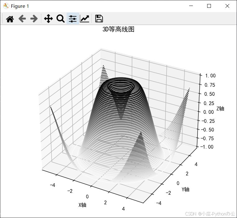
x = np. linspace( - 5 , 5 , 100 )
y = np. linspace( - 5 , 5 , 100 )
X, Y = np. meshgrid( x, y)
Z = np. sin( np. sqrt( X** 2 + Y** 2 ) )
fig = plt. figure( figsize= ( 12 , 8 ) )
ax = fig. add_subplot( 111 , projection= '3d' )
ax. contour3D( X, Y, Z, 50 , cmap= 'binary' )
ax. set_title( '3D等高线图' )
ax. set_xlabel( 'X轴' )
ax. set_ylabel( 'Y轴' )
ax. set_zlabel( 'Z轴' )
plt. tight_layout( )
plt. show( )
import matplotlib. pyplot as plt
from mpl_toolkits. mplot3d import Axes3D
import numpy as np
from pylab import *
mpl. rcParams[ 'font.sans-serif' ] = [ 'SimHei' ]
mpl. rcParams[ 'axes.unicode_minus' ] = False
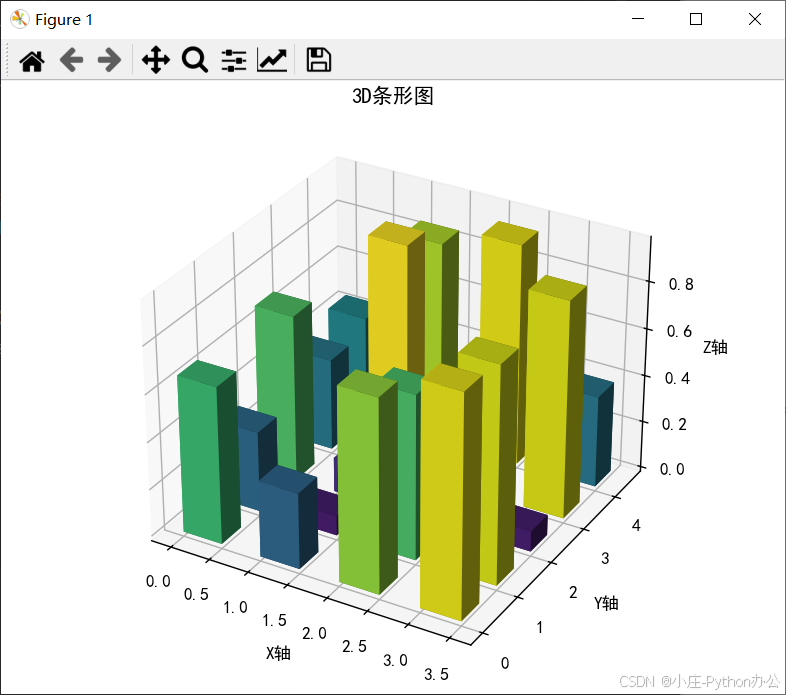
x_pos = np. arange( 4 )
y_pos = np. arange( 5 )
x_pos, y_pos = np. meshgrid( x_pos, y_pos)
x_pos = x_pos. flatten( )
y_pos = y_pos. flatten( )
z_pos = np. zeros_like( x_pos)
dx = dy = 0.5 * np. ones_like( z_pos)
dz = np. random. rand( 20 )
fig = plt. figure( figsize= ( 10 , 7 ) )
ax = fig. add_subplot( 111 , projection= '3d' )
colors = plt. cm. viridis( dz / float ( max ( dz) ) )
ax. bar3d( x_pos, y_pos, z_pos, dx, dy, dz, color= colors, shade= True )
ax. set_title( '3D条形图' )
ax. set_xlabel( 'X轴' )
ax. set_ylabel( 'Y轴' )
ax. set_zlabel( 'Z轴' )
plt. tight_layout( )
plt. show( )
import matplotlib. pyplot as plt
from mpl_toolkits. mplot3d import Axes3D
import numpy as np
from pylab import *
mpl. rcParams[ 'font.sans-serif' ] = [ 'SimHei' ]
mpl. rcParams[ 'axes.unicode_minus' ] = False
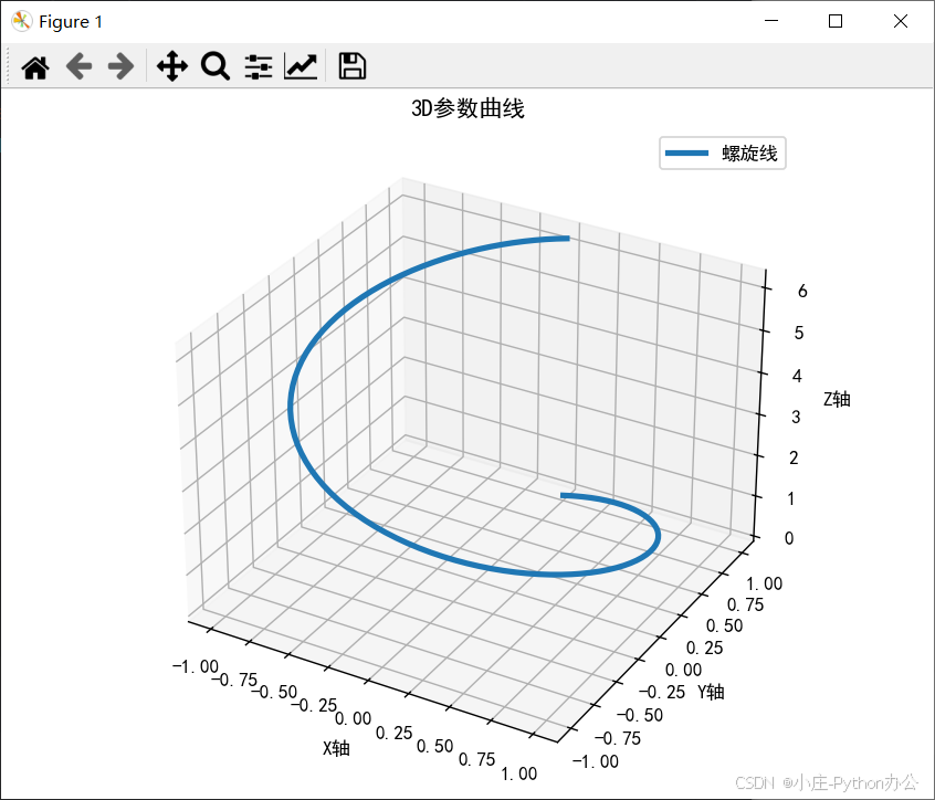
t = np. linspace( 0 , 2 * np. pi, 100 )
x = np. sin( t)
y = np. cos( t)
z = t
fig = plt. figure( figsize= ( 10 , 7 ) )
ax = fig. add_subplot( 111 , projection= '3d' )
ax. plot( x, y, z, label= '螺旋线' , linewidth= 3 )
ax. set_title( '3D参数曲线' )
ax. set_xlabel( 'X轴' )
ax. set_ylabel( 'Y轴' )
ax. set_zlabel( 'Z轴' )
ax. legend( )
plt. tight_layout( )
plt. show( )
from matplotlib. patches import Polygon
import numpy as np
from matplotlib. collections import PolyCollection
import matplotlib. pyplot as plt
from mpl_toolkits. mplot3d import Axes3D
import matplotlib as mpl
mpl. rcParams[ 'font.sans-serif' ] = [ 'SimHei' ]
mpl. rcParams[ 'axes.unicode_minus' ] = False
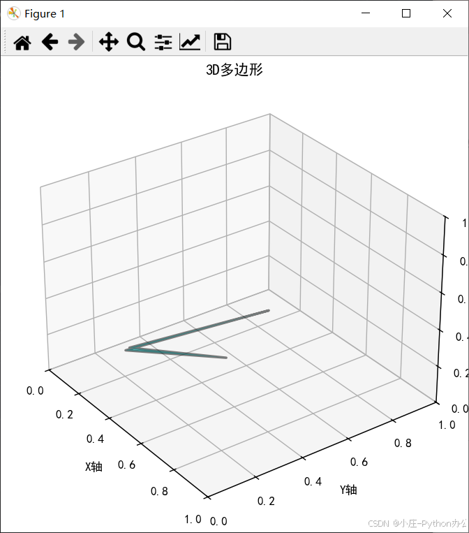
verts2d = np. random. rand( 4 , 2 )
verts3d = [ list ( map ( lambda xy: ( xy[ 0 ] , xy[ 1 ] , 0 ) , verts2d) ) ]
fig = plt. figure( figsize= ( 10 , 7 ) )
ax = fig. add_subplot( 111 , projection= '3d' )
poly3d = PolyCollection( [ verts2d] , facecolors= 'cyan' , edgecolors= 'k' , linewidths= 2 , alpha= 0.5 )
ax. add_collection3d( poly3d, zs= 0 , zdir= 'z' )
ax. set_xlim( 0 , 1 )
ax. set_ylim( 0 , 1 )
ax. set_zlim( 0 , 1 )
ax. set_title( '3D多边形' )
ax. set_xlabel( 'X轴' )
ax. set_ylabel( 'Y轴' )
ax. set_zlabel( 'Z轴' )
plt. tight_layout( )
plt. show( )
from matplotlib. patches import Polygon
import numpy as np
from matplotlib. collections import PolyCollection
import matplotlib. pyplot as plt
from mpl_toolkits. mplot3d import Axes3D
import matplotlib as mpl
mpl. rcParams[ 'font.sans-serif' ] = [ 'SimHei' ]
mpl. rcParams[ 'axes.unicode_minus' ] = False
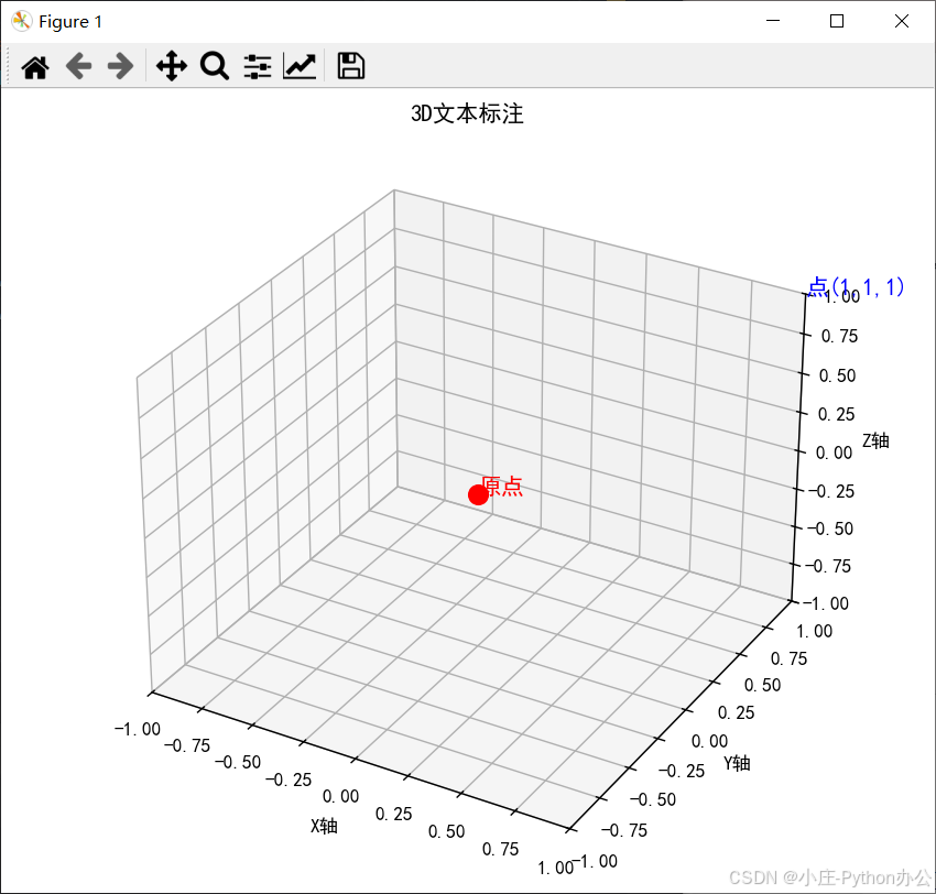
fig = plt. figure( figsize= ( 10 , 7 ) )
ax = fig. add_subplot( 111 , projection= '3d' )
ax. scatter( [ 0 ] , [ 0 ] , [ 0 ] , color= 'r' , s= 100 )
ax. text( 0 , 0 , 0 , "原点" , color= 'red' , fontsize= 12 )
ax. text( 1 , 1 , 1 , "点(1,1,1)" , color= 'blue' , fontsize= 12 )
ax. set_xlim( - 1 , 1 )
ax. set_ylim( - 1 , 1 )
ax. set_zlim( - 1 , 1 )
ax. set_title( '3D文本标注' )
ax. set_xlabel( 'X轴' )
ax. set_ylabel( 'Y轴' )
ax. set_zlabel( 'Z轴' )
plt. tight_layout( )
plt. show( )
import numpy as np
import matplotlib. pyplot as plt
from matplotlib. animation import FuncAnimation
from pylab import *
mpl. rcParams[ 'font.sans-serif' ] = [ 'SimHei' ]
mpl. rcParams[ 'axes.unicode_minus' ] = False
def get_3d_data ( t) :
theta = np. linspace( - 4 * np. pi, 4 * np. pi, 100 )
z = np. linspace( - 2 , 2 , 100 )
r = z** 2 + 1 + 0.5 * np. sin( t)
x = r * np. sin( theta + t/ 10 )
y = r * np. cos( theta + t/ 10 )
return x, y, z
fig = plt. figure( figsize= ( 10 , 7 ) )
ax = fig. add_subplot( 111 , projection= '3d' )
line, = ax. plot( [ ] , [ ] , [ ] , lw= 2 )
ax. set_xlim( - 5 , 5 )
ax. set_ylim( - 5 , 5 )
ax. set_zlim( - 2 , 2 )
ax. set_title( '3D动画' )
ax. set_xlabel( 'X轴' )
ax. set_ylabel( 'Y轴' )
ax. set_zlabel( 'Z轴' )
def update ( t) :
x, y, z = get_3d_data( t)
line. set_data( x, y)
line. set_3d_properties( z)
return line,
ani = FuncAnimation( fig, update, frames= 100 , interval= 50 , blit= True )
plt. tight_layout( )
plt. show( )
希望对初学者有帮助 致力于办公自动化的小小程序员一枚 希望能得到大家的【一个免费关注】!感谢 求个 🤞 关注 🤞 求个 ❤️ 喜欢 ❤️ 求个 👍 收藏 👍


 1523
1523

 被折叠的 条评论
为什么被折叠?
被折叠的 条评论
为什么被折叠?
 到【灌水乐园】发言


