SIFT算法

SIFT算法

特点

1、具有较好的稳定性和不变性，能够适应旋转、尺度缩放、亮度的变化，能在一定程度上不受视角变化、仿射变换、噪声的干扰。
2、区分性好，能够在海量特征数据库中进行快速准确的区分信息进行匹配
3、多量性，就算只有单个物体，也能产生大量特征向量
4、高速性，能够快速的进行特征向量匹配
5、可扩展性，能够与其它形式的特征向量进行联合

实质

算法步骤

1、提取关键点：关键点是一些十分突出的不会因光照、尺度、旋转等因素而消失的点，比如角点、边缘点、暗区域的亮点以及亮区域的暗点。此步骤是搜索所有尺度空间上的图像位置。通过高斯微分函数来识别潜在的具有尺度和旋转不变的兴趣点。
2、定位关键点并确定特征方向：在每个候选的位置上，通过一个拟合精细的模型来确定位置和尺度。关键点的选择依据于它们的稳定程度。然后基于图像局部的梯度方向，分配给每个关键点位置一个或多个方向。所有后面的对图像数据的操作都相对于关键点的方向、尺度和位置进行变换，从而提供对于这些变换的不变性。
3. 通过各关键点的特征向量，进行两两比较找出相互匹配的若干对特征点，建立景物间的对应关系。

关于RANSAC算法

概述

RANSAC算法的输入是一组观测数据，一个可以解释或者适应于观测数据的参数化模型，一些可信的参数。

RANSAC通过反复选择数据中的一组随机子集来达成目标。被选取的子集被假设为局内点，并用下述方法进行验证：
1.首先我们先随机假设一小组局内点为初始值。然后用此局内点拟合一个模型，此模型适应于假设的局内点，所有的未知参数都能从假设的局内点计算得出。
2.用1中得到的模型去测试所有的其它数据，如果某个点适用于估计的模型，认为它也是局内点，将局内点扩充。
3.如果有足够多的点被归类为假设的局内点，那么估计的模型就足够合理。
4.然后，用所有假设的局内点去重新估计模型，因为此模型仅仅是在初始的假设的局内点估计的，后续有扩充后，需要更新。
5.最后，通过估计局内点与模型的错误率来评估模型。

整个这个过程为迭代一次，此过程被重复执行固定的次数，每次产生的模型有两个结局：
1、要么因为局内点太少，还不如上一次的模型，而被舍弃，
2、要么因为比现有的模型更好而被选用。

算法步骤

2. 计算数据集中所有数据与模型M的投影误差，若误差小于阈值，加入内点集 I ；

3. 如果当前内点集 I 元素个数大于最优内点集 I_best , 则更新 I_best = I，同时更新迭代次数k ;

4. 如果迭代次数大于k,则退出 ; 否则迭代次数加1，并重复上述步骤；

优点与缺点

RANSAC的优点是它能鲁棒的估计模型参数。例如，它能从包含大量局外点的数据集中估计出高精度的参数。

RANSAC的缺点是它计算参数的迭代次数没有上限；如果设置迭代次数的上限，得到的结果可能不是最优的结果，甚至可能得到错误的结果。RANSAC只有一定的概率得到可信的模型，概率与迭代次数成正比。RANSAC的另一个缺点是它要求设置跟问题相关的阀值。

RANSAC只能从特定的数据集中估计出一个模型，如果存在两个（或多个）模型，RANSAC不能找到别的模型。

实验

1、准备数据集

2、对每张图片进行SIFT特征提取，并展示特征点

2.1、代码

# -*- coding: utf-8 -*-
from PIL import Image
from pylab import *
from PCV.localdescriptors import sift

# 添加中文字体支持
from matplotlib.font_manager import FontProperties
font = FontProperties(fname=r"c:\windows\fonts\SimSun.ttc", size=14)

imname = 'data/15.jpg'
im = array(Image.open(imname).convert('L'))
sift.process_image(imname, 'empire.sift')
l1, d1 = sift.read_features_from_file('empire.sift')

figure()
gray()
subplot(121)
sift.plot_features(im, l1, circle=False)
title(u'SIFT特征',fontproperties=font)
subplot(122)
sift.plot_features(im, l1, circle=True)
title(u'用圆圈表示SIFT特征尺度',fontproperties=font)

show()

2.2、实验结果

1.jgp

2.jpg

3.jpg

4.jpg

5.jpg

6.jpg

7.jpg

8.jpg

9.jpg

10.jpg

11.jpg

12.jpg

13.jpg

14.jpg

15.jpg

2.3、实验小结

1、检测速度非常快

2、检测效率高，检测特征点数量比Harris丰富

3、检测精确度非常高

3、给定任意两张图片，计算SIFT匹配结果

3.1、代码

# -*- coding: utf-8 -*-
from pylab import *
from PIL import Image

from PCV.localdescriptors import harris
from PCV.tools.imtools import imresize

"""
This is the Harris point matching example in Figure 2-2.
"""

im1 = array(Image.open("data/1.jpg").convert("L"))
im2 = array(Image.open("data/2.jpg").convert("L"))

# resize加快匹配速度
im1 = imresize(im1, (im1.shape[1]//2, im1.shape[0]//2))
im2 = imresize(im2, (im2.shape[1]//2, im2.shape[0]//2))

wid = 5
harrisim = harris.compute_harris_response(im1, 5)
filtered_coords1 = harris.get_harris_points(harrisim, wid+1)
d1 = harris.get_descriptors(im1, filtered_coords1, wid)

harrisim = harris.compute_harris_response(im2, 5)
filtered_coords2 = harris.get_harris_points(harrisim, wid+1)
d2 = harris.get_descriptors(im2, filtered_coords2, wid)

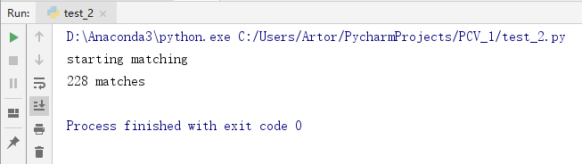
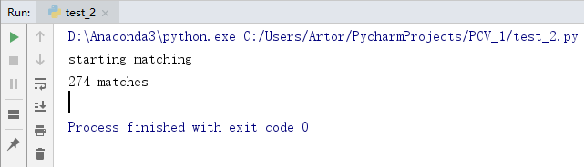
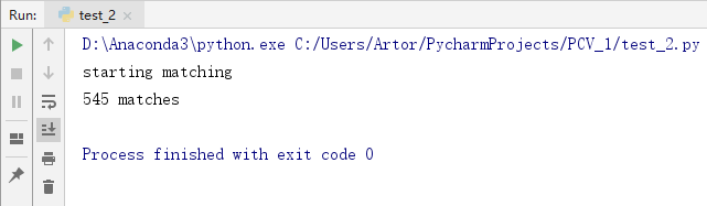
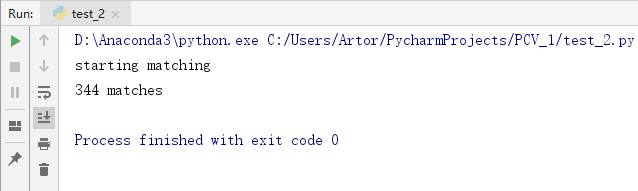
print ('starting matching')
matches = harris.match_twosided(d1, d2)

print('{} matches'.format(len(matches.nonzero()[0])))

figure()
gray() 
harris.plot_matches(im1, im2, filtered_coords1, filtered_coords2, matches)
show()

3.2、实验结果

第一组

第二组

第三组

第四组

3.3 实验小结

1、匹配速度非常快

2、对物体匹配不受背景杂物噪声的影响，匹配很精确

3、对物体拍摄的图像进行角度变化、光照变化、尺度变化等，发现并不会影响SIFT匹配，而且非常精确，图片匹配度也很高，说明SIFT算法是一个很优秀的算法

4、给定一张输入图片，在数据集内部搜索匹配最多的三张图片

4.1 代码

# -*- coding: utf-8 -*-
from PIL import Image
from pylab import *
from numpy import *
import os
from PCV.tools.imtools import get_imlist  # 导入原书的PCV模块
import matplotlib.pyplot as plt  # plt 用于显示图片
import matplotlib.image as mpimg  # mpimg 用于读取图片
 
 
def process_image(imagename, resultname, params="--edge-thresh 10 --peak-thresh 5"):
    """ 处理一幅图像，然后将结果保存在文件中"""
    if imagename[-3:] != 'pgm':
        # 创建一个pgm文件
        im = Image.open(imagename).convert('L')
        im.save('tmp.pgm')
        imagename = 'tmp.pgm'
    cmmd = str("sift " + imagename + " --output=" + resultname + " " + params)
    os.system(cmmd)
    print 'processed', imagename, 'to', resultname
 
 
def read_features_from_file(filename):
    """读取特征属性值，然后将其以矩阵的形式返回"""
    f = loadtxt(filename)
    return f[:, :4], f[:, 4:]  # 特征位置，描述子
 
 
def write_featrues_to_file(filename, locs, desc):
    """将特征位置和描述子保存到文件中"""
    savetxt(filename, hstack((locs, desc)))
 
 
def plot_features(im, locs, circle=False):
    """显示带有特征的图像
       输入：im（数组图像），locs（每个特征的行、列、尺度和朝向）"""
 
    def draw_circle(c, r):
        t = arange(0, 1.01, .01) * 2 * pi
        x = r * cos(t) + c[0]
        y = r * sin(t) + c[1]
        plot(x, y, 'b', linewidth=2)
 
    imshow(im)
    if circle:
        for p in locs:
            draw_circle(p[:2], p[2])
    else:
        plot(locs[:, 0], locs[:, 1], 'ob')
    axis('off')
 
 
def match(desc1, desc2):
    """对于第一幅图像中的每个描述子，选取其在第二幅图像中的匹配
    输入：desc1(第一幅图像中的描述子)，desc2(第二幅图像中的描述子)"""
    desc1 = array([d / linalg.norm(d) for d in desc1])
    desc2 = array([d / linalg.norm(d) for d in desc2])
    dist_ratio = 0.6
    desc1_size = desc1.shape
    matchscores = zeros((desc1_size[0], 1), 'int')
    desc2t = desc2.T  # 预先计算矩阵转置
    for i in range(desc1_size[0]):
        dotprods = dot(desc1[i, :], desc2t)  # 向量点乘
        dotprods = 0.9999 * dotprods
        # 反余弦和反排序，返回第二幅图像中特征的索引
        indx = argsort(arccos(dotprods))
        # 检查最近邻的角度是否小于dist_ratio乘以第二近邻的角度
        if arccos(dotprods)[indx[0]] < dist_ratio * arccos(dotprods)[indx[1]]:
            matchscores[i] = int(indx[0])
    return matchscores
 
 
def match_twosided(desc1, desc2):
    """双向对称版本的match()"""
    matches_12 = match(desc1, desc2)
    matches_21 = match(desc2, desc1)
    ndx_12 = matches_12.nonzero()[0]
    # 去除不对称的匹配
    for n in ndx_12:
        if matches_21[int(matches_12[n])] != n:
            matches_12[n] = 0
    return matches_12
 
 
def appendimages(im1, im2):
    """返回将两幅图像并排拼接成的一幅新图像"""
    # 选取具有最少行数的图像，然后填充足够的空行
    rows1 = im1.shape[0]
    rows2 = im2.shape[0]
    if rows1 < rows2:
        im1 = concatenate((im1, zeros((rows2 - rows1, im1.shape[1]))), axis=0)
    elif rows1 > rows2:
        im2 = concatenate((im2, zeros((rows1 - rows2, im2.shape[1]))), axis=0)
    return concatenate((im1, im2), axis=1)
 
 
def plot_matches(im1, im2, locs1, locs2, matchscores, show_below=True):
    """ 显示一幅带有连接匹配之间连线的图片
        输入：im1, im2(数组图像), locs1,locs2（特征位置）,matchscores(match()的输出)，
        show_below（如果图像应该显示在匹配的下方）
    """
    im3 = appendimages(im1, im2)
    if show_below:
        im3 = vstack((im3, im3))
    imshow(im3)
    cols1 = im1.shape[1]
    for i in range(len(matchscores)):
        if matchscores[i] > 0:
            plot([locs1[i, 0], locs2[matchscores[i, 0], 0] + cols1], [locs1[i, 1], locs2[matchscores[i, 0], 1]], 'c')
    axis('off')
 
 
# 获取project2_data文件夹下的图片文件名(包括后缀名)
filelist = get_imlist('C:\Users\Artor\PycharmProjects\PCV_1\data')
 
# 输入的图片
im1f = 'C:\Users\Artor\PycharmProjects\PCV_1\data\1.jpg'
im1 = array(Image.open(im1f))
process_image(im1f, 'out_sift_1.txt')
l1, d1 = read_features_from_file('out_sift_1.txt')
 
i = 0
num = [0] * 30  # 存放匹配值
for infile in filelist:  # 对文件夹下的每张图片进行如下操作
    im2 = array(Image.open(infile))
    process_image(infile, 'out_sift_2.txt')
    l2, d2 = read_features_from_file('out_sift_2.txt')
    matches = match_twosided(d1, d2)
    num[i] = len(matches.nonzero()[0])
    i = i + 1
    print '{} matches'.format(num[i - 1])  # 输出匹配值
 
i = 1
figure()
while i < 4:  # 循环三次，输出匹配最多的三张图片
    index = num.index(max(num))
    print index, filelist[index]
    lena = mpimg.imread(filelist[index])  # 读取当前匹配最大值的图片
    # 此时 lena 就已经是一个 np.array 了，可以对它进行任意处理
    # lena.shape  # (512, 512, 3)
    subplot(1, 3, i)
    plt.imshow(lena)  # 显示图片
    plt.axis('off')  # 不显示坐标轴
    num[index] = 0  # 将当前最大值清零
    i = i + 1
show()
 
 

4.2、实验步骤与结果

1、输入图片

2、输出三张匹配度最高图片

4.3、实验小结

1、将输入图片与数据集中每一张图片进行SIFT匹配并保留匹配值；对匹配值进行由大到小排列，并对前三进行图像的输出

2、输入一个手表的正面图片，位于整体的左上角；输出了三张匹配度最高的图片，分别是手表的左视图，正视图和右视图，输出非常准确

3、虽然只有15张图片，但是仍可以看出SIFT算法匹配速度非常快，而且结果也很精确，说明尺度变化、亮度变化、旋转等对SIFT算法影响非常小，是一种非常优秀的算法

5、匹配地理标记图像

首先通过图像间是否具有匹配的局部描述子来定义图像间的连接，然后可视化这些连接情况。为了完成可视化，我们可以在图中显示这些图像，图的边代表连接。 可以使用pydot。

为了创建显示可能图像组的图，如果匹配的数目高于一个阈值，我们使用边来连接相应的图像节点。为了得到图中的图像，需要使用图像的全路径（在下面例子中，使用 path 变量表示0）。为了使图像看起来更好看，我们需要将每幅图像尺度化为缩略图形式，缩略图的最大边为 100 像素。

5.1、代码

# -*- coding: utf-8 -*-
from pylab import *
from PIL import Image
from PCV.localdescriptors import sift
from PCV.tools import imtools
import pydot


download_path = "C:\\Users\\Artor\\PycharmProjects\\PCV_1\\data"
path = "C:\\Users\\Artor\\PycharmProjects\\PCV_1\\data"

imlist = imtools.get_imlist(download_path)
nbr_images = len(imlist)

featlist = [imname[:-3] + 'sift' for imname in imlist]
for i, imname in enumerate(imlist):
    sift.process_image(imname, featlist[i])

matchscores = zeros((nbr_images, nbr_images))

for i in range(nbr_images):
    for j in range(i, nbr_images):  # only compute upper triangle
        print('comparing ', imlist[i], imlist[j])
        l1, d1 = sift.read_features_from_file(featlist[i])
        l2, d2 = sift.read_features_from_file(featlist[j])
        matches = sift.match_twosided(d1, d2)
        nbr_matches = sum(matches > 0)
        print('number of matches = ', nbr_matches)
        matchscores[i, j] = nbr_matches

# copy values
for i in range(nbr_images):
    for j in range(i + 1, nbr_images):  # no need to copy diagonal
        matchscores[j, i] = matchscores[i, j]

# 可视化

threshold = 2  # min number of matches needed to create link

g = pydot.Dot(graph_type='graph')  # don't want the default directed graph

for i in range(nbr_images):
    for j in range(i + 1, nbr_images):
        if matchscores[i, j] > threshold:
            # first image in pair
            im = Image.open(imlist[i])
            im.thumbnail((100, 100))
            filename = path + str(i) + '.jpg'
            im.save(filename)  # need temporary files of the right size
            g.add_node(pydot.Node(str(i), fontcolor='transparent', shape='rectangle', image=filename))

            # second image in pair
            im = Image.open(imlist[j])
            im.thumbnail((100, 100))
            filename = path + str(j) + '.jpg'
            im.save(filename)  # need temporary files of the right size
            g.add_node(pydot.Node(str(j), fontcolor='transparent', shape='rectangle', image=filename))

            g.add_edge(pydot.Edge(str(i), str(j)))

g.write_jpg('C:\\Users\\Artor\\PycharmProjects\\PCV_1\\data\\TEST.jpg')

5.2、实验步骤与结果

1、对数据集中每张图片进行SIFT特征提取并保存提取结果

2、以第一张图为主，与数据集中其他每一张图进行匹配，输出匹配结果

3、对数据集中每一张图都与其他每张图进行匹配（即重复步骤2），已匹配的跳过

4、对最后结果进行可视化连接输出

5.3、实验小结

1、数据集中存在15张图片，最多只需匹配105次；即数据集中存在n张图片，最多只需匹配（n*(n-1)/2）次。匹配次数少，匹配速度也非常快

2、将数据集中图片匹配结果可视化，将相同物体存在的图片进行连接，数据集图片分类情况清晰明确，结果一目了然

3、可以将图像之间的匹配数进行输出，也可根据可视化连接进行图像之间匹配数的查询，使结果更具体

4、数据集共有4种不同物品的15张图片，通过本次实验可以快速进行图片分类与关系表示，简洁明了；算法整体运行速度快，无论角度、尺度、光照变化，关系连线都非常准确，进一步说明了SIFT算法的优越性

6、RANSAC算法应用

6.1、代码

# -*- coding: utf-8
from pylab import *
from numpy import *
from PIL import Image
from scipy.spatial import Delaunay
# If you have PCV installed, these imports should work
from PCV.geometry import homography, warp
from PCV.localdescriptors import sift



"""
This is the panorama example from section 3.3.
"""

# set paths to data folder

featname = ['C:\Users\Artor\PycharmProjects\PCV_1\data\' + str(i + 1) + '.sift' for i in range(5)]
imname = ['C:\Users\Artor\PycharmProjects\PCV_1\data\' + str(i + 1) + '.jpg' for i in range(5)]

# extract features and match
l = {}
d = {}
for i in range(5):
    sift.process_image(imname[i], featname[i])
    l[i], d[i] = sift.read_features_from_file(featname[i])

matches = {}
for i in range(4):
    matches[i] = sift.match(d[i + 1], d[i])

# visualize the matches (Figure 3-11 in the book)
# sift匹配可视化
for i in range(4):
    im1 = array(Image.open(imname[i]))
    im2 = array(Image.open(imname[i + 1]))
    figure()
    sift.plot_matches(im2, im1, l[i + 1], l[i], matches[i], show_below=True)


# function to convert the matches to hom. points
# 将匹配转换成齐次坐标点的函数
def convert_points(j):
    ndx = matches[j].nonzero()[0]
    fp = homography.make_homog(l[j + 1][ndx, :2].T)
    ndx2 = [int(matches[j][i]) for i in ndx]
    tp = homography.make_homog(l[j][ndx2, :2].T)

    # switch x and y - TODO this should move elsewhere
    fp = vstack([fp[1], fp[0], fp[2]])
    tp = vstack([tp[1], tp[0], tp[2]])
    return fp, tp


# estimate the homographies
# 估计单应性矩阵
model = homography.RansacModel()

fp, tp = convert_points(1)
H_12 = homography.H_from_ransac(fp, tp, model)[0]  # im 1 to 2  # im1 到 im2 的单应性矩阵


fp, tp = convert_points(0)
H_01 = homography.H_from_ransac(fp, tp, model)[0]  # im 0 to 1

tp, fp = convert_points(2)  # NB: reverse order
H_32 = homography.H_from_ransac(fp, tp, model)[0]  # im 3 to 2

tp, fp = convert_points(3)  # NB: reverse order
H_43 = homography.H_from_ransac(fp, tp, model)[0]  # im 4 to 3

# warp the images
# 扭曲图像

delta = 2000  # for padding and translation 用于填充和平移

im1 = array(Image.open(imname[1]), "uint8")
im2 = array(Image.open(imname[2]), "uint8")
im_12 = warp.panorama(H_12, im1, im2, delta, delta)

im1 = array(Image.open(imname[0]), "f")
im_02 = warp.panorama(dot(H_12, H_01), im1, im_12, delta, delta)

im1 = array(Image.open(imname[3]), "f")
im_32 = warp.panorama(H_32, im1, im_02, delta, delta)

im1 = array(Image.open(imname[4]), "f")
im_42 = warp.panorama(dot(H_32, H_43), im1, im_32, delta, 2 * delta)
imsave('xxx.jpg', array(im_42, "uint8"))
figure()
imshow(array(im_42, "uint8"))
axis('off')
show()

6.2、实验结果

1、景深单一场景


2、景深丰富场景

6.3、实验小结

在单一的图片场景中，在没有进行RANSAC算法剔除错误匹配之前，出现了较多的匹配错误的情况，进行RANSAC算法剔除错误匹配之后，虽然剔除掉了许多错误匹配，但同时也将正确的匹配点剔除掉，还是存在一定的误差。

在景深丰富场景中，可以看出在未进行RANSAC算法剔除错误之前，匹配出的结果较多，线条也非常凌乱，出现的错配的情况也较多，在进行RANSAC算法剔除错误后，两幅图片匹配出来的结果比较准确，错配的情况还是存在，但较未进行RANSAC算法剔除错误之前，错配情况减少了许多，准确度提高了不少。

结论

1、SIFT算法具有丰富的特征点检测，精确度很高，而且检测速度非常快

2、对物体拍摄的图像进行角度变化、光照变化、尺度变化等，不会影响SIFT匹配

3、相较于Harris算法，在速度与效率上明显更强，是一个很优秀的算法

4、仍然存在一定缺点：实时性不高、有时特征点较少、 对边缘光滑的目标无法准确提取特征点。