Meta人体AI模型 Sapiens：High-resolution models for human tasks

本文链接：https://blog.csdn.net/weixin_42744466/article/details/144555451

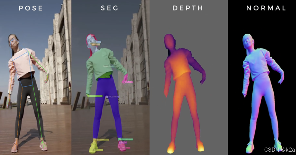
Meta公司一直是图像和视频模型开发的先锋，最近他们推出了一项名为Meta Sapiens的新模型，专注于与人类相关的任务。与Homo sapiens（智人）相似，Meta Sapiens模型旨在理解和模拟人类行为，包括理解身体姿势、识别身体部位、预测深度，甚至确定皮肤纹理等表面细节。本文将详细解析Meta Sapiens模型的三大支柱、技术实现以及代码实践。
在这里插入图片描述

Meta Sapiens 的三大支柱

Meta Sapiens模型的核心在于三个关键品质：泛化、广泛适用和高保真度。

泛化：模型能够在多种不同情况下表现良好，包括不同的光照条件、相机角度和各类衣物。
广泛适用：模型能够执行多种任务，如姿势估计、身体部位识别和距离预测，无需大的改动。
高保真度：模型能够创建高质量、详细的结果，如逼真的3D人体模型，具有清晰的面部特征和身体形状。

技术实现

Meta Sapiens模型使用了一些强大的技术来实现这些任务，包括MAE（蒙版自动编码器）和关键点及分割技术。

MAE（蒙版自动编码器）：通过查看缺少部分的图像并尝试填补空白，使模型更好地理解图像并节省训练时间。
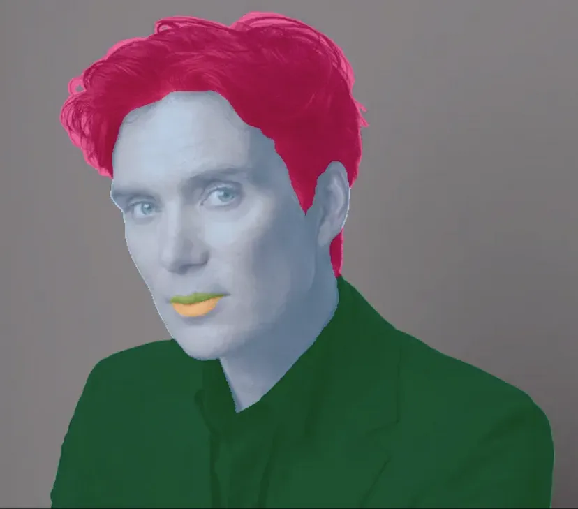
关键点和分割：模型识别人体上的308个点，包括手、脚、脸和躯干，并知道约28个不同的身体部位，从头发到嘴唇再到四肢，非常详细。

2D 姿势估计

2D姿势估计任务要求模型猜测关键身体部位的位置。该模型通过创建“热图”来工作，显示身体部位在特定位置的可能性。

架构

输入：图像 $\in R^{H×W×3}$ ，其中H为高度，W为宽度。
步骤1：重新缩放图像 — 输入图像被调整为固定高度H和宽度W。
步骤2：姿势估计变换器§ — 变换器模型处理图像以预测关键点位置。
步骤3：损失函数（均方误差） — 使用均方误差(MSE)计算预测的热图与实际位置的差异。
步骤4：编码器-解码器架构 — 使用预训练的权重初始化编码器，而解码器则随机初始化。

代码实现

以下是姿势估计的代码实现，包括模型加载、图像预处理、关键点检测和可视化。

# 模型加载
TASK = 'pose'
VERSION = 'sapiens_1b'
model_path = get_model_path(TASK, VERSION)
print(model_path)

# 图像预处理和姿势估计
def get_pose(image, pose_estimator, input_shape=(3, 1024, 768), device="cuda"):
    # Preprocess the image
    img = preprocess_image(image, input_shape)
    
    # Run the model
    with torch.no_grad():
        heatmap = pose_estimator(img.to(device))
    
    # Post-process the output
    keypoints, keypoint_scores = udp_decode(heatmap[0].cpu().float().numpy(), 
                                            input_shape[1:], 
                                            (input_shape[1] // 4, input_shape[2] // 4))
    
    # Scale keypoints to original image size
    scale_x = image.width / input_shape[2]
    scale_y = image.height / input_shape[1]
    keypoints[:, 0] *= scale_x
    keypoints[:, 1] *= scale_y
    
    # Visualize the keypoints on the original image
    pose_image = visualize_keypoints(image, keypoints, keypoint_scores)
    return pose_image
 
def preprocess_image(image, input_shape):
    # Resize and normalize the image
    img = image.resize((input_shape[2], input_shape[1]))
    img = np.array(img).transpose(2, 0, 1)
    img = torch.from_numpy(img).float()
    img = img[[2, 1, 0], ...] # RGB to BGR
    mean = torch.tensor([123.675, 116.28, 103.53]).view(3, 1, 1)
    std = torch.tensor([58.395, 57.12, 57.375]).view(3, 1, 1)
    img = (img - mean) / std
    return img.unsqueeze(0)
 
def udp_decode(heatmap, img_size, heatmap_size):
    # This is a simplified version. You might need to implement the full UDP decode logic
    h, w = heatmap_size
    keypoints = np.zeros((heatmap.shape[0], 2))
    keypoint_scores = np.zeros(heatmap.shape[0])
    
    for i in range(heatmap.shape[0]):
        hm = heatmap[i]
        idx = np.unravel_index(np.argmax(hm), hm.shape)
        keypoints[i] = [idx[1] * img_size[1] / w, idx[0] * img_size[0] / h]
        keypoint_scores[i] = hm[idx]
    
    return keypoints, keypoint_scores
 
def visualize_keypoints(image, keypoints, keypoint_scores, threshold=0.3):
    draw = ImageDraw.Draw(image)
    for (x, y), score in zip(keypoints, keypoint_scores):
        if score > threshold:
            draw.ellipse([(x-2, y-2), (x+2, y+2)], fill='red', outline='red')
    return image

身体部位分割

身体部位分割任务中，模型对图像中的每个像素进行分类，将其分解为手臂、腿或脸等身体部位。

架构

输入：图像 $\in R^{H×W×3}$ 。
步骤1：编码器-解码器架构 — 身体部位分割模型遵循与姿势估计相同的编码器-解码器设置。
步骤2：像素分类 — 模型将图像的每个像素分类为C个身体部位类别之一。
步骤3：损失函数（加权交叉熵） — 使用加权交叉熵损失进行微调。

代码实现

以下是身体部位分割的代码实现，包括模型加载、图像预处理和可视化。

# 模型加载
def get_model_path(task, version):
    try:
        model_path = SAPIENS_LITE_MODELS_PATH[task][version]
        if not os.path.exists(model_path):
            print(f"Warning: The model file does not exist at {model_path}")
        return model_path
    except KeyError as e:
        print(f"Error: Invalid task or version. {e}")
        return None

TASK = 'seg'
VERSION = 'sapiens_0.3b'
model_path = get_model_path(TASK, VERSION)
print(model_path)

# 图像分割
def segment(image):
    input_tensor = transform_fn(image).unsqueeze(0).to("cuda")
    preds = run_model(input_tensor, height=image.height, width=image.width)
    mask = preds.squeeze(0).cpu().numpy()
    mask_image = Image.fromarray(mask.astype("uint8"))
    blended_image = visualize_mask_with_overlay(image, mask_image, LABELS_TO_IDS, alpha=0.5)
    return blended_image

身体部位分割结果
人体分割结果

深度估计

深度估计任务有助于模型了解图像不同部分的距离，这对于增强现实等任务很重要。

架构

输入：图像 $\in R^{H×W×3}$ 。
步骤1：编码器-解码器架构 — 编码器从图像中提取特征，解码器预测每个像素的深度。
步骤2：单通道深度图 — 输出通道设置为1，生成深度图。
步骤3：损失函数（回归） — 将预测的深度值与地面实况进行比较，并使用回归损失最小化差异。

代码实现

以下是深度估计的代码实现，包括模型加载、图像预处理和可视化。

# 模型加载
TASK = 'depth'
VERSION = 'sapiens_0.3b'
model_path = get_model_path(TASK, VERSION)
print(model_path)

def get_depth(image, depth_model, input_shape=(3, 1024, 768), device="cuda"):
    # Preprocess the image
    img = preprocess_image(image, input_shape)
    
    # Run the model
    with torch.no_grad():
        result = depth_model(img.to(device))
    
    # Post-process the output
    depth_map = post_process_depth(result, (image.shape[0], image.shape[1]))
    
    # Visualize the depth map
    depth_image = visualize_depth(depth_map)
    
    return depth_image, depth_map
 
def preprocess_image(image, input_shape):
    img = cv2.resize(image, (input_shape[2], input_shape[1]), interpolation=cv2.INTER_LINEAR).transpose(2, 0, 1)
    img = torch.from_numpy(img)
    img = img[[2, 1, 0], ...].float()
    mean = torch.tensor([123.5, 116.5, 103.5]).view(-1, 1, 1)
    std = torch.tensor([58.5, 57.0, 57.5]).view(-1, 1, 1)
    img = (img - mean) / std
    return img.unsqueeze(0)
 
def post_process_depth(result, original_shape):
    # Check the dimensionality of the result
    if result.dim() == 3:
        result = result.unsqueeze(0)
    elif result.dim() == 4:
        pass
    else:
        raise ValueError(f"Unexpected result dimension: {result.dim()}")
    
    # Ensure we're interpolating to the correct dimensions
    seg_logits = F.interpolate(result, size=original_shape, mode="bilinear", align_corners=False).squeeze(0)
    depth_map = seg_logits.data.float().cpu().numpy()
    
    # If depth_map has an extra dimension, squeeze it
    if depth_map.ndim == 3 and depth_map.shape[0] == 1:
        depth_map = depth_map.squeeze(0)
    
    return depth_map
def visualize_depth(depth_map):
    # Normalize the depth map
    min_val, max_val = np.nanmin(depth_map), np.nanmax(depth_map)
    depth_normalized = 1 - ((depth_map - min_val) / (max_val - min_val))
    
    # Convert to uint8
    depth_normalized = (depth_normalized * 255).astype(np.uint8)
    
    # Apply colormap
    depth_colored = cv2.applyColorMap(depth_normalized, cv2.COLORMAP_INFERNO)
    
    return depth_colored
    
# You can add the surface normal calculation if needed
def calculate_surface_normal(depth_map):
    kernel_size = 7
    grad_x = cv2.Sobel(depth_map.astype(np.float32), cv2.CV_32F, 1, 0, ksize=kernel_size)
    grad_y = cv2.Sobel(depth_map.astype(np.float32), cv2.CV_32F, 0, 1, ksize=kernel_size)
    z = np.full(grad_x.shape, -1)
    normals = np.dstack((-grad_x, -grad_y, z))
    normals_mag = np.linalg.norm(normals, axis=2, keepdims=True)
    with np.errstate(divide="ignore", invalid="ignore"):
        normals_normalized = normals / (normals_mag + 1e-5)
    normals_normalized = np.nan_to_num(normals_normalized, nan=-1, posinf=-1, neginf=-1)
    normal_from_depth = ((normals_normalized + 1) / 2 * 255).astype(np.uint8)
    normal_from_depth = normal_from_depth[:, :, ::-1]  # RGB to BGR for cv2
    return normal_from_depth

表面法线估计

表面法线估计任务让模型找出人体的3D表面细节，例如每个点的表面角度或方向。

架构

输入：图像（I ∈ R^H×W×3）。
步骤1：编码器-解码器架构 — 法线估计模型使用编码器-解码器框架。
步骤2：表面法线的三通道输出 — 解码器输出通道设置为3，对应于法线矢量的xyz分量。
步骤3：损失函数（余弦相似度） — 使用L1损失和余弦相似度的组合来比较预测的法线向量与地面真实法线。

代码实现

以下是表面法线估计的代码实现，包括模型加载、图像预处理和可视化。

# 模型加载
TASK = 'normal'
VERSION = 'sapiens_0.3b'
model_path = get_model_path(TASK, VERSION)
print(model_path)

# 图像法线估计
def get_normal(image, normal_model, input_shape=(3, 1024, 768), device="cuda"):
    # Preprocess the image
    img = preprocess_image(image, input_shape)
    # Run the model
    with torch.no_grad():
        result = normal_model(img.to(device))
    # Post-process the output
    normal_map = post_process_normal(result, (image.shape[0], image.shape[1]))
    # Visualize the normal map
    normal_image = visualize_normal(normal_map)
    return normal_image, normal_map
 
def preprocess_image(image, input_shape):
    img = cv2.resize(image, (input_shape[2], input_shape[1]), interpolation=cv2.INTER_LINEAR).transpose(2, 0, 1)
    img = torch.from_numpy(img)
    img = img[[2, 1, 0], ...].float()
    mean = torch.tensor([123.5, 116.5, 103.5]).view(-1, 1, 1)
    std = torch.tensor([58.5, 57.0, 57.5]).view(-1, 1, 1)
    img = (img - mean) / std
    return img.unsqueeze(0)
 
def post_process_normal(result, original_shape):
    # Check the dimensionality of the result
    if result.dim() == 3:
        result = result.unsqueeze(0)
    elif result.dim() == 4:
        pass
    else:
        raise ValueError(f"Unexpected result dimension: {result.dim()}")
    
    # Ensure we're interpolating to the correct dimensions
    seg_logits = F.interpolate(result, size=original_shape, mode="bilinear", align_corners=False).squeeze(0)
    normal_map = seg_logits.float().cpu().numpy().transpose(1, 2, 0)  # H x W x 3
    return normal_map
def visualize_normal(normal_map):
    normal_map_norm = np.linalg.norm(normal_map, axis=-1, keepdims=True)
    normal_map_normalized = normal_map / (normal_map_norm + 1e-5)  # Add a small epsilon to avoid division by zero
    
    # Convert to 0-255 range and BGR format for visualization
    normal_map_vis = ((normal_map_normalized + 1) / 2 * 255).astype(np.uint8)
    normal_map_vis = normal_map_vis[:, :, ::-1]  # RGB to BGR
    
    return normal_map_vis
def load_normal_model(checkpoint, use_torchscript=False):
    if use_torchscript:
        return torch.jit.load(checkpoint)
    else:
        model = torch.export.load(checkpoint).module()
        model = model.to("cuda")
        model = torch.compile(model, mode="max-autotune", fullgraph=True)
        return model

结束语

尽管Meta Sapiens在理解与人类相关的任务方面表现出色，但它在更复杂的场景中也面临挑战。例如，当多个人站得很近（拥挤）或个人摆出不寻常或罕见的姿势时，模型很难准确估计姿势并分割身体部位。此外，严重的遮挡——当身体的某些部位被遮挡时——进一步增加了模型提供精确结果的能力。

Meta Sapiens代表了以人为本的人工智能向前迈出的重要一步，在姿势估计、分割、深度预测和表面法线估计方面提供了强大的功能。然而，与许多模型一样，它仍然存在局限性，特别是在拥挤或高度复杂的场景中。随着人工智能的不断发展，像Sapiens这样的模型的未来迭代有望解决这些挑战，使我们更接近更准确、更可靠的以人为本的应用程序。

原文链接：Meta Sapiens 人体AI模型