科研绘图之R语言生存分析KM曲线累计风险表放在图片内部

KM估计

KM估计同时利用生存时间（连续变量）和生存结局（一般为分类变量，用来表示状态）信息，是一种求生存时间函数，即S(t)的方法。

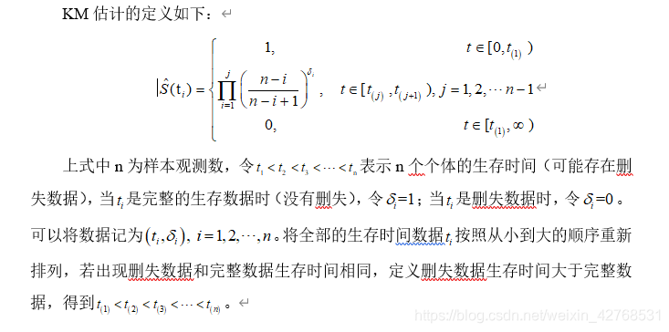
KM估计的定义如下：

R语言展示KM估计的生存函数曲线

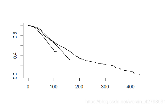
1、最简单的方法

在R里，有多种实现方法，最简单的就是

# An highlighted block
library(survival)
#创建一个生存对象，duration_Mup表示生存时间变量，这里是一个连续数值变量，status表示生存结局变量，我这里的是一个虚拟变量，0表示右删失，1表示死亡。entrystage表示感兴趣的影响生存的变量，这里是一个分类变量，数字1,2,3分别表示一种类型，data_new是所用的数据集
city<-survfit(Surv(duration_Mup,status)~entrystage,data=data_new)
plot(city)

2、利用survminer包绘制

library(survminer)
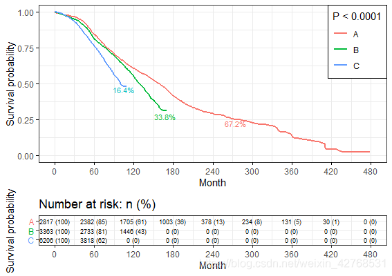
A <-ggsurvplot(city, data = data_new, 
                     ggtheme = theme_bw(),pval = T,
                     break.time.by=60,censor=FALSE, 
                     xlim = c(0, 480),
                     legend.labs=c("A", "B","C"))+
  xlab("Month") + ylab("Survival probability")
A

pval = T是log-rank对数秩检验结果，可以看出p值小于0.1%，表明A、B、C三组间的生存函数存在显著差异；
ggtheme = theme_bw()，直接调用了theme_bw()的主题；
break.time.by=60，将X轴刻度按60分隔开；
xlim = c(0, 480)，控制X轴显示范围；
censor=FALSE，不显示删失点

3、进一步美化，添加累计风险表格、图例、文本注释

library(survminer)
B <-ggsurvplot(city, data = data.frame(data_new), 
                     ggtheme = theme_bw(),
                     break.time.by=60,censor=FALSE, legend.title="P < 0.0001",
                     risk.table = "abs_pct",
                     risk.table.fontsize=2.5,tables.height=0.3,
                     xlim = c(0, 480),
                     legend.labs=c("A", "B","C"))+
  xlab("Month") + ylab("Survival probability")

B$plot <- B$plot+ 
  theme(legend.background = element_rect(fill="white",colour = "black"),
        legend.position = c(1,1),legend.justification = c(1,1))+
  ggplot2::annotate("text", x =168, y = 0.27,
                    label = "33.8%",colour="#00BA38", size = 3)+
  ggplot2::annotate("text", x = 105, y = 0.46,
                    label = "16.4%",colour="#00BFC4", size = 3)+
  ggplot2::annotate("text",x = 275, y = 0.22,
                    label = "67.2%", colour="#F8766D",size = 3)
  
B

pval = T是log-rank对数秩检验结果，可以看出p值小于0.1%，表明A、B、C三组间的生存函数存在显著差异；
ggtheme = theme_bw()，直接调用了theme_bw()的主题；
break.time.by=60，将X轴刻度按60分隔开；
xlim = c(0, 480)，控制X轴显示范围；
censor=FALSE，不显示删失点

C <-ggsurvplot(fit, data = lung, fun = "event",
                     ggtheme = theme_bw(),
                     break.time.by=60,censor=FALSE, legend.title="P < 0.0001",
                     risk.table = "absolute",risk.table.pos=c("in"),
                     risk.table.fontsize=2.5,tables.height=0.2,
                     legend.labs=c("Male", "Female"))+
  xlab("Month") + ylab("Survival probability")

C$plot <- C$plot+ 
  theme(legend.background = element_rect(fill="white",colour = "black"),
        legend.position = c(1,1),legend.justification = c(1,1))+
  ggplot2::annotate("text",x = 10, y = 0.14,
                    label = "No.at risk", colour="black",size = 4)
C

进一步美化: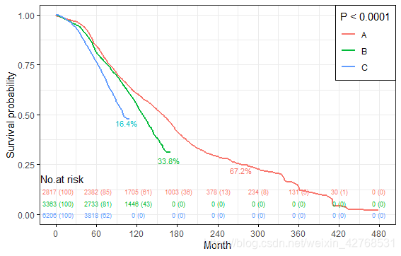

最后给大家分享基本有关生存分析的精选书籍，感兴趣的朋友欢迎加qq 782222801互相学习交流进步，谢谢！

[1]: Allison Paul D. Survival Analysis Using SAS®: A Practical Guide [M]. Sas Institute, 2010.
[2]: Kleinbaum David G., Klein Mitchel. Survival Analysis: A Self‐Learning Text [M]. Third ed. New York, NY: Springer-Verlag, 2012.