3 pandas

最新推荐文章于 2024-04-30 19:24:04 发布

唯羽

最新推荐文章于 2024-04-30 19:24:04 发布

阅读量1k

点赞数

分类专栏： python机器学习(科学计算库) 文章标签： python 机器学习 pandas

本文链接：https://blog.csdn.net/weixin_42871902/article/details/103249970

版权

python机器学习(科学计算库) 专栏收录该内容

3 篇文章 0 订阅

订阅专栏

1 pandas介绍

以Numpy为基础，借力numpy模块在计算方面性能高的优势

基于matplotlib，能够简便的画图

独特的数据结构

1.1 案例

import pandas as pd
import numpy as np

stock_change = np.random.normal(0, 1, (10, 5))
stock_change

array([[-1.0098501 ,  0.91625883,  0.10632482,  0.79909581,  1.02338447],
       [ 0.10041493,  0.85587085, -0.22404526, -0.61776538, -0.62323357],
       [ 0.70700457,  1.62502952, -0.97157201,  0.1988851 ,  0.79445365],
       [ 1.75233775, -1.17758937,  1.49103167,  0.21690815,  2.89886016],
       [ 0.05850193,  0.03554848, -0.48183573,  0.59494259,  1.08469151],
       [-0.99142601,  0.96349396,  0.26639733,  0.80381255, -0.36345471],
       [ 0.21497035, -0.53030381,  0.22778879,  1.74725041,  0.20228056],
       [ 0.1410646 ,  0.69803466, -1.24066274,  0.10367728, -1.41174687],
       [-0.3225248 ,  0.4897488 , -0.9790225 , -0.76514549,  2.00229418],
       [-0.02618594, -0.59289681,  0.89586171,  1.10466512, -0.53421044]])

# 使用pandas中的数据结构
stock_day_rise = pd.DataFrame(stock_change)
stock_day_rise

	0	1	2	3	4
0	-1.009850	0.916259	0.106325	0.799096	1.023384
1	0.100415	0.855871	-0.224045	-0.617765	-0.623234
2	0.707005	1.625030	-0.971572	0.198885	0.794454
3	1.752338	-1.177589	1.491032	0.216908	2.898860
4	0.058502	0.035548	-0.481836	0.594943	1.084692
5	-0.991426	0.963494	0.266397	0.803813	-0.363455
6	0.214970	-0.530304	0.227789	1.747250	0.202281
7	0.141065	0.698035	-1.240663	0.103677	-1.411747
8	-0.322525	0.489749	-0.979023	-0.765145	2.002294
9	-0.026186	-0.592897	0.895862	1.104665	-0.534210

# 增加行索引
stock_code = ['股票' + str(i+1) for i in range(stock_day_rise.shape[0])]
data = pd.DataFrame(stock_change, index=stock_code)
data

	0	1	2	3	4
股票1	-1.009850	0.916259	0.106325	0.799096	1.023384
股票2	0.100415	0.855871	-0.224045	-0.617765	-0.623234
股票3	0.707005	1.625030	-0.971572	0.198885	0.794454
股票4	1.752338	-1.177589	1.491032	0.216908	2.898860
股票5	0.058502	0.035548	-0.481836	0.594943	1.084692
股票6	-0.991426	0.963494	0.266397	0.803813	-0.363455
股票7	0.214970	-0.530304	0.227789	1.747250	0.202281
股票8	0.141065	0.698035	-1.240663	0.103677	-1.411747
股票9	-0.322525	0.489749	-0.979023	-0.765145	2.002294
股票10	-0.026186	-0.592897	0.895862	1.104665	-0.534210

# 增加列索引, 'B'略过周末
date = pd.date_range('2017-01-01', periods=stock_day_rise.shape[1], freq='B')
data = pd.DataFrame(stock_change, index=stock_code, columns=date)
data

	2017-01-02	2017-01-03	2017-01-04	2017-01-05	2017-01-06
股票1	-1.009850	0.916259	0.106325	0.799096	1.023384
股票2	0.100415	0.855871	-0.224045	-0.617765	-0.623234
股票3	0.707005	1.625030	-0.971572	0.198885	0.794454
股票4	1.752338	-1.177589	1.491032	0.216908	2.898860
股票5	0.058502	0.035548	-0.481836	0.594943	1.084692
股票6	-0.991426	0.963494	0.266397	0.803813	-0.363455
股票7	0.214970	-0.530304	0.227789	1.747250	0.202281
股票8	0.141065	0.698035	-1.240663	0.103677	-1.411747
股票9	-0.322525	0.489749	-0.979023	-0.765145	2.002294
股票10	-0.026186	-0.592897	0.895862	1.104665	-0.534210

1.2 DataFrame的属性

data.shape

(10, 5)

data.index

Index(['股票1', '股票2', '股票3', '股票4', '股票5', '股票6', '股票7', '股票8', '股票9', '股票10'], dtype='object')

data.columns

DatetimeIndex(['2017-01-02', '2017-01-03', '2017-01-04', '2017-01-05',
               '2017-01-06'],
              dtype='datetime64[ns]', freq='B')

data.values

array([[-1.0098501 ,  0.91625883,  0.10632482,  0.79909581,  1.02338447],
       [ 0.10041493,  0.85587085, -0.22404526, -0.61776538, -0.62323357],
       [ 0.70700457,  1.62502952, -0.97157201,  0.1988851 ,  0.79445365],
       [ 1.75233775, -1.17758937,  1.49103167,  0.21690815,  2.89886016],
       [ 0.05850193,  0.03554848, -0.48183573,  0.59494259,  1.08469151],
       [-0.99142601,  0.96349396,  0.26639733,  0.80381255, -0.36345471],
       [ 0.21497035, -0.53030381,  0.22778879,  1.74725041,  0.20228056],
       [ 0.1410646 ,  0.69803466, -1.24066274,  0.10367728, -1.41174687],
       [-0.3225248 ,  0.4897488 , -0.9790225 , -0.76514549,  2.00229418],
       [-0.02618594, -0.59289681,  0.89586171,  1.10466512, -0.53421044]])

data.T

	股票1	股票2	股票3	股票4	股票5	股票6	股票7	股票8	股票9	股票10
2017-01-02	-1.009850	0.100415	0.707005	1.752338	0.058502	-0.991426	0.214970	0.141065	-0.322525	-0.026186
2017-01-03	0.916259	0.855871	1.625030	-1.177589	0.035548	0.963494	-0.530304	0.698035	0.489749	-0.592897
2017-01-04	0.106325	-0.224045	-0.971572	1.491032	-0.481836	0.266397	0.227789	-1.240663	-0.979023	0.895862
2017-01-05	0.799096	-0.617765	0.198885	0.216908	0.594943	0.803813	1.747250	0.103677	-0.765145	1.104665
2017-01-06	1.023384	-0.623234	0.794454	2.898860	1.084692	-0.363455	0.202281	-1.411747	2.002294	-0.534210

# 默认五条
data.head()

	2017-01-02	2017-01-03	2017-01-04	2017-01-05	2017-01-06
股票1	-1.009850	0.916259	0.106325	0.799096	1.023384
股票2	0.100415	0.855871	-0.224045	-0.617765	-0.623234
股票3	0.707005	1.625030	-0.971572	0.198885	0.794454
股票4	1.752338	-1.177589	1.491032	0.216908	2.898860
股票5	0.058502	0.035548	-0.481836	0.594943	1.084692

data.tail()

	2017-01-02	2017-01-03	2017-01-04	2017-01-05	2017-01-06
股票6	-0.991426	0.963494	0.266397	0.803813	-0.363455
股票7	0.214970	-0.530304	0.227789	1.747250	0.202281
股票8	0.141065	0.698035	-1.240663	0.103677	-1.411747
股票9	-0.322525	0.489749	-0.979023	-0.765145	2.002294
股票10	-0.026186	-0.592897	0.895862	1.104665	-0.534210

1.3 DataFrame索引的设置

stock_code = ['股票_' + str(i + 1) for i in range(stock_day_rise.shape[0])]
# 必须整体全部修改
data.index = stock_code
data

	2017-01-02	2017-01-03	2017-01-04	2017-01-05	2017-01-06
股票_1	-1.009850	0.916259	0.106325	0.799096	1.023384
股票_2	0.100415	0.855871	-0.224045	-0.617765	-0.623234
股票_3	0.707005	1.625030	-0.971572	0.198885	0.794454
股票_4	1.752338	-1.177589	1.491032	0.216908	2.898860
股票_5	0.058502	0.035548	-0.481836	0.594943	1.084692
股票_6	-0.991426	0.963494	0.266397	0.803813	-0.363455
股票_7	0.214970	-0.530304	0.227789	1.747250	0.202281
股票_8	0.141065	0.698035	-1.240663	0.103677	-1.411747
股票_9	-0.322525	0.489749	-0.979023	-0.765145	2.002294
股票_10	-0.026186	-0.592897	0.895862	1.104665	-0.534210

# 重置索引
data.reset_index()

	index	2017-01-02 00:00:00	2017-01-03 00:00:00	2017-01-04 00:00:00	2017-01-05 00:00:00	2017-01-06 00:00:00
0	股票_1	-1.009850	0.916259	0.106325	0.799096	1.023384
1	股票_2	0.100415	0.855871	-0.224045	-0.617765	-0.623234
2	股票_3	0.707005	1.625030	-0.971572	0.198885	0.794454
3	股票_4	1.752338	-1.177589	1.491032	0.216908	2.898860
4	股票_5	0.058502	0.035548	-0.481836	0.594943	1.084692
5	股票_6	-0.991426	0.963494	0.266397	0.803813	-0.363455
6	股票_7	0.214970	-0.530304	0.227789	1.747250	0.202281
7	股票_8	0.141065	0.698035	-1.240663	0.103677	-1.411747
8	股票_9	-0.322525	0.489749	-0.979023	-0.765145	2.002294
9	股票_10	-0.026186	-0.592897	0.895862	1.104665	-0.534210

# drop=True
data.reset_index(drop=True)

	2017-01-02	2017-01-03	2017-01-04	2017-01-05	2017-01-06
0	-1.009850	0.916259	0.106325	0.799096	1.023384
1	0.100415	0.855871	-0.224045	-0.617765	-0.623234
2	0.707005	1.625030	-0.971572	0.198885	0.794454
3	1.752338	-1.177589	1.491032	0.216908	2.898860
4	0.058502	0.035548	-0.481836	0.594943	1.084692
5	-0.991426	0.963494	0.266397	0.803813	-0.363455
6	0.214970	-0.530304	0.227789	1.747250	0.202281
7	0.141065	0.698035	-1.240663	0.103677	-1.411747
8	-0.322525	0.489749	-0.979023	-0.765145	2.002294
9	-0.026186	-0.592897	0.895862	1.104665	-0.534210

# 以某列值设置为新的索引
df = pd.DataFrame({'month': [1, 4, 7, 10],
                    'year': [2012, 2012, 2013, 2013],
                    'sale':[55, 40, 84, 31]})
df

	month	year	sale
0	1	2012	55
1	4	2012	40
2	7	2013	84
3	10	2013	31

df.set_index('month')

	year	sale
month
1	2012	55
4	2012	40
7	2013	84
10	2013	31

# 设置多索引
new_df = df.set_index(['year', 'month'])
new_df

		sale
year	month
2012	1	55
2012	4	40
2013	7	84
2013	10	31

1.4 Multilndex与Panel

# Multilndex
new_df.index.names

FrozenList(['year', 'month'])

new_df.index.levels

FrozenList([[2012, 2013], [1, 4, 7, 10]])

new_df['sale']

year  month
2012  1        55
      4        40
2013  7        84
      10       31
Name: sale, dtype: int64

new_df['sale'][2012][1]

# Panel 新版被废弃了
# p = pd.Panel(np.arange(24).reshape(4,3,2),
#             items=list('ABCD'),
#             major_axis=pd.date_range('20130101', periods=3),
#             minor_axis=['first', 'second'])
# p

1.5 Series结构

type(data['2017-01-02'])

pandas.core.series.Series

data['2017-01-02']['股票_1']

-1.0098501036527945

# 创建series
pd.Series(np.arange(10))

0    0
1    1
2    2
3    3
4    4
5    5
6    6
7    7
8    8
9    9
dtype: int64

pd.Series([6.7,5.6,3,10,2], index=[1,2,3,4,5])

1     6.7
2     5.6
3     3.0
4    10.0
5     2.0
dtype: float64

s = pd.Series({'red':100, 'blue': 200, 'green': 500, 'yellow': 1000})

s.index

Index(['red', 'blue', 'green', 'yellow'], dtype='object')

s.values

array([ 100,  200,  500, 1000])

2 基本数据操作

data = pd.read_csv('./data/stock_day.csv')
data

	open	high	close	low	volume	price_change	p_change	ma5	ma10	ma20	v_ma5	v_ma10	v_ma20	turnover
2018-02-27	23.53	25.88	24.16	23.53	95578.03	0.63	2.68	22.942	22.142	22.875	53782.64	46738.65	55576.11	2.39
2018-02-26	22.80	23.78	23.53	22.80	60985.11	0.69	3.02	22.406	21.955	22.942	40827.52	42736.34	56007.50	1.53
2018-02-23	22.88	23.37	22.82	22.71	52914.01	0.54	2.42	21.938	21.929	23.022	35119.58	41871.97	56372.85	1.32
2018-02-22	22.25	22.76	22.28	22.02	36105.01	0.36	1.64	21.446	21.909	23.137	35397.58	39904.78	60149.60	0.90
2018-02-14	21.49	21.99	21.92	21.48	23331.04	0.44	2.05	21.366	21.923	23.253	33590.21	42935.74	61716.11	0.58
...	...	...	...	...	...	...	...	...	...	...	...	...	...	...
2015-03-06	13.17	14.48	14.28	13.13	179831.72	1.12	8.51	13.112	13.112	13.112	115090.18	115090.18	115090.18	6.16
2015-03-05	12.88	13.45	13.16	12.87	93180.39	0.26	2.02	12.820	12.820	12.820	98904.79	98904.79	98904.79	3.19
2015-03-04	12.80	12.92	12.90	12.61	67075.44	0.20	1.57	12.707	12.707	12.707	100812.93	100812.93	100812.93	2.30
2015-03-03	12.52	13.06	12.70	12.52	139071.61	0.18	1.44	12.610	12.610	12.610	117681.67	117681.67	117681.67	4.76
2015-03-02	12.25	12.67	12.52	12.20	96291.73	0.32	2.62	12.520	12.520	12.520	96291.73	96291.73	96291.73	3.30

643 rows × 14 columns

data = data.drop(['ma5', 'ma10', 'ma20', 'v_ma5', 'v_ma10', 'v_ma20'], axis=1)
data

	open	high	close	low	volume	price_change	p_change	turnover
2018-02-27	23.53	25.88	24.16	23.53	95578.03	0.63	2.68	2.39
2018-02-26	22.80	23.78	23.53	22.80	60985.11	0.69	3.02	1.53
2018-02-23	22.88	23.37	22.82	22.71	52914.01	0.54	2.42	1.32
2018-02-22	22.25	22.76	22.28	22.02	36105.01	0.36	1.64	0.90
2018-02-14	21.49	21.99	21.92	21.48	23331.04	0.44	2.05	0.58
...	...	...	...	...	...	...	...	...
2015-03-06	13.17	14.48	14.28	13.13	179831.72	1.12	8.51	6.16
2015-03-05	12.88	13.45	13.16	12.87	93180.39	0.26	2.02	3.19
2015-03-04	12.80	12.92	12.90	12.61	67075.44	0.20	1.57	2.30
2015-03-03	12.52	13.06	12.70	12.52	139071.61	0.18	1.44	4.76
2015-03-02	12.25	12.67	12.52	12.20	96291.73	0.32	2.62	3.30

643 rows × 8 columns

2.1 索引操作

# 直接使用行列索引（先列后行）
data['open']['2018-02-27']

23.53

# 结合loc或者iloc使用索引
data.loc['2018-02-27': '2018-02-22', 'open']

2018-02-27    23.53
2018-02-26    22.80
2018-02-23    22.88
2018-02-22    22.25
Name: open, dtype: float64

data.iloc[0:100, 0:1].head()

	open
2018-02-27	23.53
2018-02-26	22.80
2018-02-23	22.88
2018-02-22	22.25
2018-02-14	21.49

# 使用ix组合索引
data.ix[0:4, ['open', 'close', 'high', 'low']]

/Users/admin/.virtualenvs/ai/lib/python3.7/site-packages/ipykernel_launcher.py:2: FutureWarning: 
.ix is deprecated. Please use
.loc for label based indexing or
.iloc for positional indexing

See the documentation here:
http://pandas.pydata.org/pandas-docs/stable/user_guide/indexing.html#ix-indexer-is-deprecated
  
/Users/admin/.virtualenvs/ai/lib/python3.7/site-packages/pandas/core/indexing.py:822: FutureWarning: 
.ix is deprecated. Please use
.loc for label based indexing or
.iloc for positional indexing

See the documentation here:
http://pandas.pydata.org/pandas-docs/stable/user_guide/indexing.html#ix-indexer-is-deprecated
  retval = getattr(retval, self.name)._getitem_axis(key, axis=i)

	open	close	high	low
2018-02-27	23.53	24.16	25.88	23.53
2018-02-26	22.80	23.53	23.78	22.80
2018-02-23	22.88	22.82	23.37	22.71
2018-02-22	22.25	22.28	22.76	22.02

2.2 赋值操作

data['close'] = 1

data

	open	high	close	low	volume	price_change	p_change	turnover
2018-02-27	23.53	25.88	1	23.53	95578.03	0.63	2.68	2.39
2018-02-26	22.80	23.78	1	22.80	60985.11	0.69	3.02	1.53
2018-02-23	22.88	23.37	1	22.71	52914.01	0.54	2.42	1.32
2018-02-22	22.25	22.76	1	22.02	36105.01	0.36	1.64	0.90
2018-02-14	21.49	21.99	1	21.48	23331.04	0.44	2.05	0.58
...	...	...	...	...	...	...	...	...
2015-03-06	13.17	14.48	1	13.13	179831.72	1.12	8.51	6.16
2015-03-05	12.88	13.45	1	12.87	93180.39	0.26	2.02	3.19
2015-03-04	12.80	12.92	1	12.61	67075.44	0.20	1.57	2.30
2015-03-03	12.52	13.06	1	12.52	139071.61	0.18	1.44	4.76
2015-03-02	12.25	12.67	1	12.20	96291.73	0.32	2.62	3.30

643 rows × 8 columns

data.close = 2

data

	open	high	close	low	volume	price_change	p_change	turnover
2018-02-27	23.53	25.88	2	23.53	95578.03	0.63	2.68	2.39
2018-02-26	22.80	23.78	2	22.80	60985.11	0.69	3.02	1.53
2018-02-23	22.88	23.37	2	22.71	52914.01	0.54	2.42	1.32
2018-02-22	22.25	22.76	2	22.02	36105.01	0.36	1.64	0.90
2018-02-14	21.49	21.99	2	21.48	23331.04	0.44	2.05	0.58
...	...	...	...	...	...	...	...	...
2015-03-06	13.17	14.48	2	13.13	179831.72	1.12	8.51	6.16
2015-03-05	12.88	13.45	2	12.87	93180.39	0.26	2.02	3.19
2015-03-04	12.80	12.92	2	12.61	67075.44	0.20	1.57	2.30
2015-03-03	12.52	13.06	2	12.52	139071.61	0.18	1.44	4.76
2015-03-02	12.25	12.67	2	12.20	96291.73	0.32	2.62	3.30

643 rows × 8 columns

2.3 排序

data.sort_values(by='p_change', ascending=False).head()

	open	high	close	low	volume	price_change	p_change	turnover
2015-08-28	15.40	16.46	2	15.00	117827.60	1.50	10.03	4.03
2015-05-21	27.50	28.22	2	26.50	121190.11	2.57	10.02	4.15
2016-12-22	18.50	20.42	2	18.45	150470.83	1.86	10.02	3.77
2015-08-04	16.20	17.35	2	15.80	94292.63	1.58	10.02	3.23
2016-07-07	18.66	18.66	2	18.41	48756.55	1.70	10.02	1.67

data.sort_values(by=['open', 'high']).head()

	open	high	close	low	volume	price_change	p_change	turnover
2015-03-02	12.25	12.67	2	12.20	96291.73	0.32	2.62	3.30
2015-09-02	12.30	14.11	2	12.30	70201.74	-1.10	-8.17	2.40
2015-03-03	12.52	13.06	2	12.52	139071.61	0.18	1.44	4.76
2015-03-04	12.80	12.92	2	12.61	67075.44	0.20	1.57	2.30
2015-03-05	12.88	13.45	2	12.87	93180.39	0.26	2.02	3.19

data.sort_index()

	open	high	close	low	volume	price_change	p_change	turnover
2015-03-02	12.25	12.67	2	12.20	96291.73	0.32	2.62	3.30
2015-03-03	12.52	13.06	2	12.52	139071.61	0.18	1.44	4.76
2015-03-04	12.80	12.92	2	12.61	67075.44	0.20	1.57	2.30
2015-03-05	12.88	13.45	2	12.87	93180.39	0.26	2.02	3.19
2015-03-06	13.17	14.48	2	13.13	179831.72	1.12	8.51	6.16
...	...	...	...	...	...	...	...	...
2018-02-14	21.49	21.99	2	21.48	23331.04	0.44	2.05	0.58
2018-02-22	22.25	22.76	2	22.02	36105.01	0.36	1.64	0.90
2018-02-23	22.88	23.37	2	22.71	52914.01	0.54	2.42	1.32
2018-02-26	22.80	23.78	2	22.80	60985.11	0.69	3.02	1.53
2018-02-27	23.53	25.88	2	23.53	95578.03	0.63	2.68	2.39

643 rows × 8 columns

data['p_change'].sort_values().head()

2015-09-01   -10.03
2015-09-14   -10.02
2016-01-11   -10.02
2015-07-15   -10.02
2015-08-26   -10.01
Name: p_change, dtype: float64

data['p_change'].sort_index().head()

2015-03-02    2.62
2015-03-03    1.44
2015-03-04    1.57
2015-03-05    2.02
2015-03-06    8.51
Name: p_change, dtype: float64

3 DataFrame运算

data['open'].add(1)

2018-02-27    24.53
2018-02-26    23.80
2018-02-23    23.88
2018-02-22    23.25
2018-02-14    22.49
              ...  
2015-03-06    14.17
2015-03-05    13.88
2015-03-04    13.80
2015-03-03    13.52
2015-03-02    13.25
Name: open, Length: 643, dtype: float64

close = data['close']
open1 = data['open']
data['m_price_change'] = close.sub(open1)

data

	open	high	close	low	volume	price_change	p_change	turnover	m_price_change
2018-02-27	23.53	25.88	2	23.53	95578.03	0.63	2.68	2.39	-21.53
2018-02-26	22.80	23.78	2	22.80	60985.11	0.69	3.02	1.53	-20.80
2018-02-23	22.88	23.37	2	22.71	52914.01	0.54	2.42	1.32	-20.88
2018-02-22	22.25	22.76	2	22.02	36105.01	0.36	1.64	0.90	-20.25
2018-02-14	21.49	21.99	2	21.48	23331.04	0.44	2.05	0.58	-19.49
...	...	...	...	...	...	...	...	...	...
2015-03-06	13.17	14.48	2	13.13	179831.72	1.12	8.51	6.16	-11.17
2015-03-05	12.88	13.45	2	12.87	93180.39	0.26	2.02	3.19	-10.88
2015-03-04	12.80	12.92	2	12.61	67075.44	0.20	1.57	2.30	-10.80
2015-03-03	12.52	13.06	2	12.52	139071.61	0.18	1.44	4.76	-10.52
2015-03-02	12.25	12.67	2	12.20	96291.73	0.32	2.62	3.30	-10.25

643 rows × 9 columns

3.1 逻辑运算符

data['p_change'] > 2

2018-02-27     True
2018-02-26     True
2018-02-23     True
2018-02-22    False
2018-02-14     True
              ...  
2015-03-06     True
2015-03-05     True
2015-03-04    False
2015-03-03    False
2015-03-02     True
Name: p_change, Length: 643, dtype: bool

# 筛选
data[data['p_change'] > 2]

	open	high	close	low	volume	price_change	p_change	turnover	m_price_change
2018-02-27	23.53	25.88	2	23.53	95578.03	0.63	2.68	2.39	-21.53
2018-02-26	22.80	23.78	2	22.80	60985.11	0.69	3.02	1.53	-20.80
2018-02-23	22.88	23.37	2	22.71	52914.01	0.54	2.42	1.32	-20.88
2018-02-14	21.49	21.99	2	21.48	23331.04	0.44	2.05	0.58	-19.49
2018-02-12	20.70	21.40	2	20.63	32445.39	0.82	4.03	0.81	-18.70
...	...	...	...	...	...	...	...	...	...
2015-03-13	14.13	14.50	2	14.08	61342.22	0.36	2.55	2.10	-12.13
2015-03-10	14.20	14.80	2	14.01	101213.51	0.34	2.38	3.46	-12.20
2015-03-06	13.17	14.48	2	13.13	179831.72	1.12	8.51	6.16	-11.17
2015-03-05	12.88	13.45	2	12.87	93180.39	0.26	2.02	3.19	-10.88
2015-03-02	12.25	12.67	2	12.20	96291.73	0.32	2.62	3.30	-10.25

183 rows × 9 columns

# 多条件
data[(data['p_change'] > 2) & (data['open'] > 15)]

	open	high	close	low	volume	price_change	p_change	turnover	m_price_change
2018-02-27	23.53	25.88	2	23.53	95578.03	0.63	2.68	2.39	-21.53
2018-02-26	22.80	23.78	2	22.80	60985.11	0.69	3.02	1.53	-20.80
2018-02-23	22.88	23.37	2	22.71	52914.01	0.54	2.42	1.32	-20.88
2018-02-14	21.49	21.99	2	21.48	23331.04	0.44	2.05	0.58	-19.49
2018-02-12	20.70	21.40	2	20.63	32445.39	0.82	4.03	0.81	-18.70
...	...	...	...	...	...	...	...	...	...
2015-04-13	19.60	21.30	2	19.50	171822.69	1.70	8.75	5.88	-17.60
2015-04-09	18.28	19.89	2	18.02	183119.05	1.20	6.51	6.27	-16.28
2015-04-08	17.60	18.53	2	17.60	157725.97	0.88	5.02	5.40	-15.60
2015-04-07	16.54	17.98	2	16.50	122471.85	0.88	5.28	4.19	-14.54
2015-03-30	15.99	16.63	2	15.99	85090.45	0.65	4.12	2.91	-13.99

161 rows × 9 columns

3.2 逻辑运算函数

data.query('p_change > 2 & turnover > 5').head()

	open	high	close	low	volume	price_change	p_change	turnover	m_price_change
2017-11-14	28.00	29.89	2	27.68	243773.23	1.10	3.90	6.10	-26.00
2017-10-31	32.62	35.22	2	32.20	361660.88	2.38	7.42	9.05	-30.62
2017-10-27	31.45	33.20	2	31.45	333824.31	0.70	2.16	8.35	-29.45
2017-10-26	29.30	32.70	2	28.92	501915.41	2.68	9.01	12.56	-27.30
2017-10-25	27.86	30.45	2	27.54	328947.31	1.68	5.99	8.23	-25.86

data[data['turnover'].isin([4.91, 2.39])]

	open	high	close	low	volume	price_change	p_change	turnover	m_price_change
2018-02-27	23.53	25.88	2	23.53	95578.03	0.63	2.68	2.39	-21.53
2016-09-28	19.88	20.98	2	19.71	95580.75	0.98	4.93	2.39	-17.88

3.3 统计运算

# 综合分析
data.describe()

	open	high	close	low	volume	price_change	p_change	turnover	m_price_change
count	643.000000	643.000000	643.0	643.000000	643.000000	643.000000	643.000000	643.000000	643.000000
mean	21.272706	21.900513	2.0	20.771835	99905.519114	0.018802	0.190280	2.936190	-19.272706
std	3.930973	4.077578	0.0	3.791968	73879.119354	0.898476	4.079698	2.079375	3.930973
min	12.250000	12.670000	2.0	12.200000	1158.120000	-3.520000	-10.030000	0.040000	-32.990000
25%	19.000000	19.500000	2.0	18.525000	48533.210000	-0.390000	-1.850000	1.360000	-21.400000
50%	21.440000	21.970000	2.0	20.980000	83175.930000	0.050000	0.260000	2.500000	-19.440000
75%	23.400000	24.065000	2.0	22.850000	127580.055000	0.455000	2.305000	3.915000	-17.000000
max	34.990000	36.350000	2.0	34.010000	501915.410000	3.030000	10.030000	12.560000	-10.250000

# 统计函数
# 求和
print(data['open'].sum())
# 平均值
print(data['open'].mean())
# 中位数
print(data['open'].median())
# 最小值
print(data['open'].min())
# 最大值
print(data['open'].max())
# 众数
print(data['open'].mode())
# 绝对值
print(data['open'].abs().head(2))
# 乘积
print(data['open'].head().prod())
# 标准差
print(data['open'].std())
# 方差
print(data['open'].var())
# 最大元素的索引
print(data['open'].idxmax())
# 最小元素的索引
print(data['open'].idxmin())

13678.35
21.27270606531882
21.44
12.25
34.99
0    20.85
1    21.30
2    24.10
dtype: float64
2018-02-27    23.53
2018-02-26    22.80
Name: open, dtype: float64
5869204.273732801
3.930972922511381
15.45254811751767
2015-06-15
2015-03-02

3.4 累计统计函数

# 排序
data = data.sort_index()

data

	open	high	close	low	volume	price_change	p_change	turnover	m_price_change
2015-03-02	12.25	12.67	2	12.20	96291.73	0.32	2.62	3.30	-10.25
2015-03-03	12.52	13.06	2	12.52	139071.61	0.18	1.44	4.76	-10.52
2015-03-04	12.80	12.92	2	12.61	67075.44	0.20	1.57	2.30	-10.80
2015-03-05	12.88	13.45	2	12.87	93180.39	0.26	2.02	3.19	-10.88
2015-03-06	13.17	14.48	2	13.13	179831.72	1.12	8.51	6.16	-11.17
...	...	...	...	...	...	...	...	...	...
2018-02-14	21.49	21.99	2	21.48	23331.04	0.44	2.05	0.58	-19.49
2018-02-22	22.25	22.76	2	22.02	36105.01	0.36	1.64	0.90	-20.25
2018-02-23	22.88	23.37	2	22.71	52914.01	0.54	2.42	1.32	-20.88
2018-02-26	22.80	23.78	2	22.80	60985.11	0.69	3.02	1.53	-20.80
2018-02-27	23.53	25.88	2	23.53	95578.03	0.63	2.68	2.39	-21.53

643 rows × 9 columns

# 累加
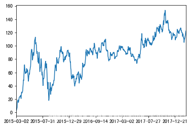
rise = data['p_change']
rise.cumsum()

2015-03-02      2.62
2015-03-03      4.06
2015-03-04      5.63
2015-03-05      7.65
2015-03-06     16.16
               ...  
2018-02-14    112.59
2018-02-22    114.23
2018-02-23    116.65
2018-02-26    119.67
2018-02-27    122.35
Name: p_change, Length: 643, dtype: float64

# 更好的显示
import matplotlib.pyplot as plt

rise.cumsum().plot()
plt.show()

在这里插入图片描述

# 最大值
rise.cummax()

2015-03-02     2.62
2015-03-03     2.62
2015-03-04     2.62
2015-03-05     2.62
2015-03-06     8.51
              ...  
2018-02-14    10.03
2018-02-22    10.03
2018-02-23    10.03
2018-02-26    10.03
2018-02-27    10.03
Name: p_change, Length: 643, dtype: float64

# 最小值
rise.cummin()

2015-03-02     2.62
2015-03-03     1.44
2015-03-04     1.44
2015-03-05     1.44
2015-03-06     1.44
              ...  
2018-02-14   -10.03
2018-02-22   -10.03
2018-02-23   -10.03
2018-02-26   -10.03
2018-02-27   -10.03
Name: p_change, Length: 643, dtype: float64

# 累乘
rise.head().cumprod()

2015-03-02      2.620000
2015-03-03      3.772800
2015-03-04      5.923296
2015-03-05     11.965058
2015-03-06    101.822643
Name: p_change, dtype: float64

3.5 自定义运算

data[['open', 'turnover']].apply(lambda x: x.max() - x.min(), axis=0)

open        22.74
turnover    12.52
dtype: float64

4 pandas画图

data.plot(figsize=(20, 8))

<matplotlib.axes._subplots.AxesSubplot at 0x115454d10>

在这里插入图片描述

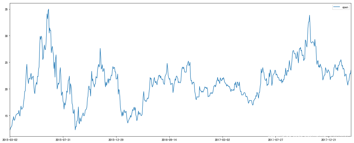
data.plot(y='open', figsize=(20, 8))

<matplotlib.axes._subplots.AxesSubplot at 0x1185caa90>

在这里插入图片描述

data.plot(x='turnover', y='open', kind='scatter', figsize=(20, 8))

<matplotlib.axes._subplots.AxesSubplot at 0x118b23850>

在这里插入图片描述

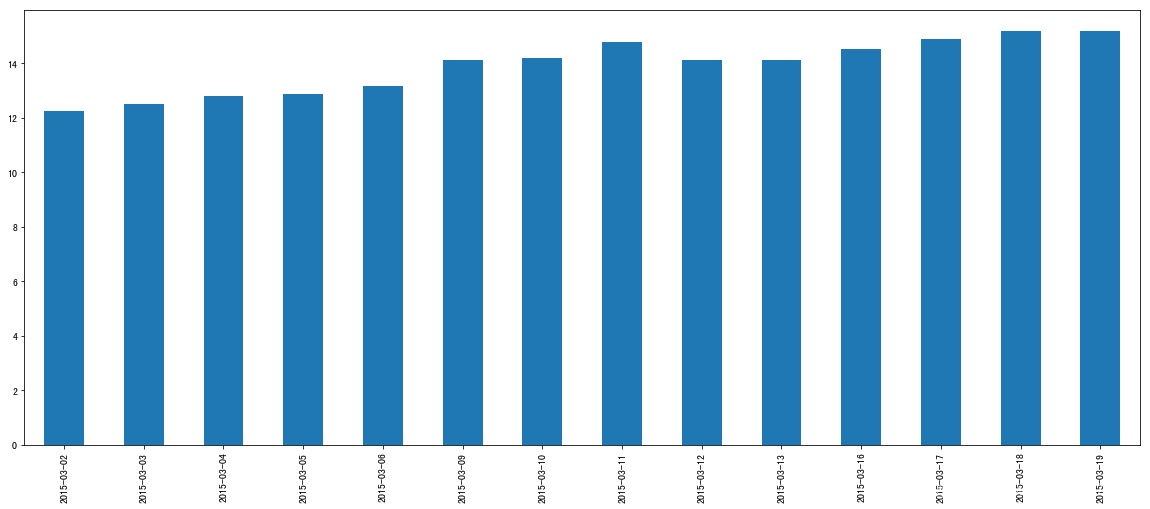
data.loc[:'2015-03-2', 'open'].plot(kind='bar', figsize=(20, 8))

<matplotlib.axes._subplots.AxesSubplot at 0x119060d10>

在这里插入图片描述

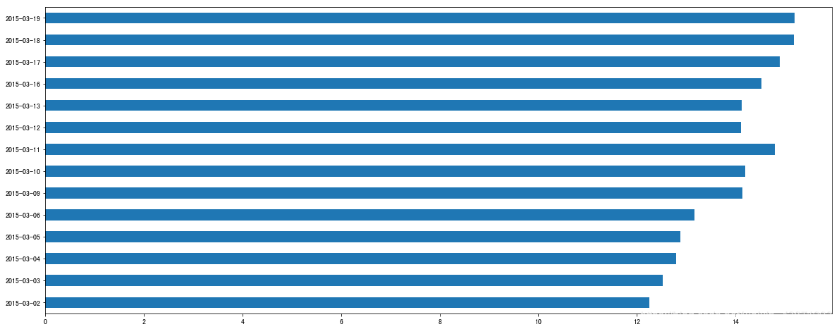
data.loc[:'2015-03-2', 'open'].plot(kind='barh', figsize=(20, 8))

<matplotlib.axes._subplots.AxesSubplot at 0x1190e9350>

在这里插入图片描述

5 文件读取与存储

5.1 csv

data = pd.read_csv('./data/stock_day.csv', usecols=['open', 'close'])

data

	open	close
2018-02-27	23.53	24.16
2018-02-26	22.80	23.53
2018-02-23	22.88	22.82
2018-02-22	22.25	22.28
2018-02-14	21.49	21.92
...	...	...
2015-03-06	13.17	14.28
2015-03-05	12.88	13.16
2015-03-04	12.80	12.90
2015-03-03	12.52	12.70
2015-03-02	12.25	12.52

643 rows × 2 columns

data[:10].to_csv('./data/test.csv', columns=['open'])

pd.read_csv('./data/test.csv')

	Unnamed: 0	open
0	2018-02-27	23.53
1	2018-02-26	22.80
2	2018-02-23	22.88
3	2018-02-22	22.25
4	2018-02-14	21.49
5	2018-02-13	21.40
6	2018-02-12	20.70
7	2018-02-09	21.20
8	2018-02-08	21.79
9	2018-02-07	22.69

# index=False不会将索引变成一列数据
data[:10].to_csv('./data/test.csv', columns=['open'], index=False)
pd.read_csv('./data/test.csv')

	open
0	23.53
1	22.80
2	22.88
3	22.25
4	21.49
5	21.40
6	20.70
7	21.20
8	21.79
9	22.69

5.2 HDF5

day = pd.read_hdf('./data/day_maxupordown.h5')
day

	000001.SZ	000002.SZ	000004.SZ	000005.SZ	000006.SZ	000007.SZ	000008.SZ	000009.SZ	000010.SZ	000011.SZ	...	001965.SZ	603283.SH	002920.SZ	002921.SZ	300684.SZ	002922.SZ	300735.SZ	603329.SH	603655.SH	603080.SH
0	1	1	0	0	0	0	0	0	0	0	...	0	0	0	0	0	0	0	0	0	0
1	0	0	0	1	0	0	0	0	0	0	...	0	0	0	0	0	0	0	0	0	0
2	0	-1	0	0	-1	0	0	-1	0	-1	...	0	0	0	0	0	0	0	0	0	0
3	0	0	0	0	0	0	0	0	0	0	...	0	0	0	0	0	0	0	0	0	0
4	0	0	0	0	0	0	0	0	0	0	...	0	0	0	0	0	0	0	0	0	0
...	...	...	...	...	...	...	...	...	...	...	...	...	...	...	...	...	...	...	...	...	...
2673	0	0	0	0	0	0	0	0	1	0	...	0	1	1	1	1	1	1	1	1	1
2674	0	0	0	0	0	0	0	0	0	0	...	0	1	0	1	1	1	1	1	1	1
2675	0	0	0	0	0	0	0	0	0	0	...	0	1	0	1	1	1	1	1	1	1
2676	0	0	0	0	0	0	0	0	0	0	...	0	1	0	0	1	0	0	1	1	1
2677	0	0	0	0	0	0	0	0	0	0	...	0	1	0	0	1	0	0	0	1	1

2678 rows × 3562 columns

day.to_hdf('./data/test.h5', key='one')

pd.read_hdf('./data/test.h5', key='one')

	000001.SZ	000002.SZ	000004.SZ	000005.SZ	000006.SZ	000007.SZ	000008.SZ	000009.SZ	000010.SZ	000011.SZ	...	001965.SZ	603283.SH	002920.SZ	002921.SZ	300684.SZ	002922.SZ	300735.SZ	603329.SH	603655.SH	603080.SH
0	1	1	0	0	0	0	0	0	0	0	...	0	0	0	0	0	0	0	0	0	0
1	0	0	0	1	0	0	0	0	0	0	...	0	0	0	0	0	0	0	0	0	0
2	0	-1	0	0	-1	0	0	-1	0	-1	...	0	0	0	0	0	0	0	0	0	0
3	0	0	0	0	0	0	0	0	0	0	...	0	0	0	0	0	0	0	0	0	0
4	0	0	0	0	0	0	0	0	0	0	...	0	0	0	0	0	0	0	0	0	0
...	...	...	...	...	...	...	...	...	...	...	...	...	...	...	...	...	...	...	...	...	...
2673	0	0	0	0	0	0	0	0	1	0	...	0	1	1	1	1	1	1	1	1	1
2674	0	0	0	0	0	0	0	0	0	0	...	0	1	0	1	1	1	1	1	1	1
2675	0	0	0	0	0	0	0	0	0	0	...	0	1	0	1	1	1	1	1	1	1
2676	0	0	0	0	0	0	0	0	0	0	...	0	1	0	0	1	0	0	1	1	1
2677	0	0	0	0	0	0	0	0	0	0	...	0	1	0	0	1	0	0	0	1	1

2678 rows × 3562 columns

5.3 json

json_read = pd.read_json('./data/columns.json', orient='records')
json_read

	article_link	headline	is_sarcastic
0	https://www.huffingtonpost.com/entry/versace-b...	former versace store clerk sues over secret 'b...	0
1	https://www.huffingtonpost.com/entry/roseanne-...	the 'roseanne' revival catches up to our thorn...	0
2	https://local.theonion.com/mom-starting-to-fea...	mom starting to fear son's web series closest ...	1
3	https://politics.theonion.com/boehner-just-wan...	boehner just wants wife to listen, not come up...	1
4	https://www.huffingtonpost.com/entry/jk-rowlin...	j.k. rowling wishes snape happy birthday in th...	0
5	https://www.huffingtonpost.com/entry/advancing...	advancing the world's women	0
6	https://www.huffingtonpost.com/entry/how-meat-...	the fascinating case for eating lab-grown meat	0
7	https://www.huffingtonpost.com/entry/boxed-col...	this ceo will send your kids to school, if you...	0
8	https://politics.theonion.com/top-snake-handle...	top snake handler leaves sinking huckabee camp...	1
9	https://www.huffingtonpost.com/entry/fridays-m...	friday's morning email: inside trump's presser...	0

json_read.to_json('./data/test.json', orient='records', lines=True)

pd.read_json('./data/test.json', lines=True)

	article_link	headline	is_sarcastic
0	https://www.huffingtonpost.com/entry/versace-b...	former versace store clerk sues over secret 'b...	0
1	https://www.huffingtonpost.com/entry/roseanne-...	the 'roseanne' revival catches up to our thorn...	0
2	https://local.theonion.com/mom-starting-to-fea...	mom starting to fear son's web series closest ...	1
3	https://politics.theonion.com/boehner-just-wan...	boehner just wants wife to listen, not come up...	1
4	https://www.huffingtonpost.com/entry/jk-rowlin...	j.k. rowling wishes snape happy birthday in th...	0
5	https://www.huffingtonpost.com/entry/advancing...	advancing the world's women	0
6	https://www.huffingtonpost.com/entry/how-meat-...	the fascinating case for eating lab-grown meat	0
7	https://www.huffingtonpost.com/entry/boxed-col...	this ceo will send your kids to school, if you...	0
8	https://politics.theonion.com/top-snake-handle...	top snake handler leaves sinking huckabee camp...	1
9	https://www.huffingtonpost.com/entry/fridays-m...	friday's morning email: inside trump's presser...	0

6 缺失值处理

6.1 判断缺失值

movie = pd.read_csv('./data/movies.csv')
movie

	Rank	Title	Genre	Description	Director	Actors	Year	Runtime (Minutes)	Rating	Votes	Revenue (Millions)	Metascore
0	1	Guardians of the Galaxy	Action,Adventure,Sci-Fi	A group of intergalactic criminals are forced ...	James Gunn	Chris Pratt, Vin Diesel, Bradley Cooper, Zoe S...	2014	121	8.1	757074	333.13	76.0
1	2	Prometheus	Adventure,Mystery,Sci-Fi	Following clues to the origin of mankind, a te...	Ridley Scott	Noomi Rapace, Logan Marshall-Green, Michael Fa...	2012	124	7.0	485820	126.46	65.0
2	3	Split	Horror,Thriller	Three girls are kidnapped by a man with a diag...	M. Night Shyamalan	James McAvoy, Anya Taylor-Joy, Haley Lu Richar...	2016	117	7.3	157606	138.12	62.0
3	4	Sing	Animation,Comedy,Family	In a city of humanoid animals, a hustling thea...	Christophe Lourdelet	Matthew McConaughey,Reese Witherspoon, Seth Ma...	2016	108	7.2	60545	270.32	59.0
4	5	Suicide Squad	Action,Adventure,Fantasy	A secret government agency recruits some of th...	David Ayer	Will Smith, Jared Leto, Margot Robbie, Viola D...	2016	123	6.2	393727	325.02	40.0
...	...	...	...	...	...	...	...	...	...	...	...	...
995	996	Secret in Their Eyes	Crime,Drama,Mystery	A tight-knit team of rising investigators, alo...	Billy Ray	Chiwetel Ejiofor, Nicole Kidman, Julia Roberts...	2015	111	6.2	27585	NaN	45.0
996	997	Hostel: Part II	Horror	Three American college students studying abroa...	Eli Roth	Lauren German, Heather Matarazzo, Bijou Philli...	2007	94	5.5	73152	17.54	46.0
997	998	Step Up 2: The Streets	Drama,Music,Romance	Romantic sparks occur between two dance studen...	Jon M. Chu	Robert Hoffman, Briana Evigan, Cassie Ventura,...	2008	98	6.2	70699	58.01	50.0
998	999	Search Party	Adventure,Comedy	A pair of friends embark on a mission to reuni...	Scot Armstrong	Adam Pally, T.J. Miller, Thomas Middleditch,Sh...	2014	93	5.6	4881	NaN	22.0
999	1000	Nine Lives	Comedy,Family,Fantasy	A stuffy businessman finds himself trapped ins...	Barry Sonnenfeld	Kevin Spacey, Jennifer Garner, Robbie Amell,Ch...	2016	87	5.3	12435	19.64	11.0

1000 rows × 12 columns

pd.notnull(movie)

	Rank	Title	Genre	Description	Director	Actors	Year	Runtime (Minutes)	Rating	Votes	Revenue (Millions)	Metascore
0	True	True	True	True	True	True	True	True	True	True	True	True
1	True	True	True	True	True	True	True	True	True	True	True	True
2	True	True	True	True	True	True	True	True	True	True	True	True
3	True	True	True	True	True	True	True	True	True	True	True	True
4	True	True	True	True	True	True	True	True	True	True	True	True
...	...	...	...	...	...	...	...	...	...	...	...	...
995	True	True	True	True	True	True	True	True	True	True	False	True
996	True	True	True	True	True	True	True	True	True	True	True	True
997	True	True	True	True	True	True	True	True	True	True	True	True
998	True	True	True	True	True	True	True	True	True	True	False	True
999	True	True	True	True	True	True	True	True	True	True	True	True

1000 rows × 12 columns

np.all(movie.isnull())

False

np.any(movie.isnull())

True

6.2 处理nan

# 不修改原数据
data = movie.dropna()
data

	Rank	Title	Genre	Description	Director	Actors	Year	Runtime (Minutes)	Rating	Votes	Revenue (Millions)	Metascore
0	1	Guardians of the Galaxy	Action,Adventure,Sci-Fi	A group of intergalactic criminals are forced ...	James Gunn	Chris Pratt, Vin Diesel, Bradley Cooper, Zoe S...	2014	121	8.1	757074	333.13	76.0
1	2	Prometheus	Adventure,Mystery,Sci-Fi	Following clues to the origin of mankind, a te...	Ridley Scott	Noomi Rapace, Logan Marshall-Green, Michael Fa...	2012	124	7.0	485820	126.46	65.0
2	3	Split	Horror,Thriller	Three girls are kidnapped by a man with a diag...	M. Night Shyamalan	James McAvoy, Anya Taylor-Joy, Haley Lu Richar...	2016	117	7.3	157606	138.12	62.0
3	4	Sing	Animation,Comedy,Family	In a city of humanoid animals, a hustling thea...	Christophe Lourdelet	Matthew McConaughey,Reese Witherspoon, Seth Ma...	2016	108	7.2	60545	270.32	59.0
4	5	Suicide Squad	Action,Adventure,Fantasy	A secret government agency recruits some of th...	David Ayer	Will Smith, Jared Leto, Margot Robbie, Viola D...	2016	123	6.2	393727	325.02	40.0
...	...	...	...	...	...	...	...	...	...	...	...	...
993	994	Resident Evil: Afterlife	Action,Adventure,Horror	While still out to destroy the evil Umbrella C...	Paul W.S. Anderson	Milla Jovovich, Ali Larter, Wentworth Miller,K...	2010	97	5.9	140900	60.13	37.0
994	995	Project X	Comedy	3 high school seniors throw a birthday party t...	Nima Nourizadeh	Thomas Mann, Oliver Cooper, Jonathan Daniel Br...	2012	88	6.7	164088	54.72	48.0
996	997	Hostel: Part II	Horror	Three American college students studying abroa...	Eli Roth	Lauren German, Heather Matarazzo, Bijou Philli...	2007	94	5.5	73152	17.54	46.0
997	998	Step Up 2: The Streets	Drama,Music,Romance	Romantic sparks occur between two dance studen...	Jon M. Chu	Robert Hoffman, Briana Evigan, Cassie Ventura,...	2008	98	6.2	70699	58.01	50.0
999	1000	Nine Lives	Comedy,Family,Fantasy	A stuffy businessman finds himself trapped ins...	Barry Sonnenfeld	Kevin Spacey, Jennifer Garner, Robbie Amell,Ch...	2016	87	5.3	12435	19.64	11.0

838 rows × 12 columns

# 替换
for i in movie.columns:
    if np.all(pd.notnull(movie[i])) == False:
        print(i)
        movie[i].fillna(movie[i].mean(), inplace=True)

Revenue (Millions)
Metascore

movie

	Rank	Title	Genre	Description	Director	Actors	Year	Runtime (Minutes)	Rating	Votes	Revenue (Millions)	Metascore
0	1	Guardians of the Galaxy	Action,Adventure,Sci-Fi	A group of intergalactic criminals are forced ...	James Gunn	Chris Pratt, Vin Diesel, Bradley Cooper, Zoe S...	2014	121	8.1	757074	333.130000	76.0
1	2	Prometheus	Adventure,Mystery,Sci-Fi	Following clues to the origin of mankind, a te...	Ridley Scott	Noomi Rapace, Logan Marshall-Green, Michael Fa...	2012	124	7.0	485820	126.460000	65.0
2	3	Split	Horror,Thriller	Three girls are kidnapped by a man with a diag...	M. Night Shyamalan	James McAvoy, Anya Taylor-Joy, Haley Lu Richar...	2016	117	7.3	157606	138.120000	62.0
3	4	Sing	Animation,Comedy,Family	In a city of humanoid animals, a hustling thea...	Christophe Lourdelet	Matthew McConaughey,Reese Witherspoon, Seth Ma...	2016	108	7.2	60545	270.320000	59.0
4	5	Suicide Squad	Action,Adventure,Fantasy	A secret government agency recruits some of th...	David Ayer	Will Smith, Jared Leto, Margot Robbie, Viola D...	2016	123	6.2	393727	325.020000	40.0
...	...	...	...	...	...	...	...	...	...	...	...	...
995	996	Secret in Their Eyes	Crime,Drama,Mystery	A tight-knit team of rising investigators, alo...	Billy Ray	Chiwetel Ejiofor, Nicole Kidman, Julia Roberts...	2015	111	6.2	27585	82.956376	45.0
996	997	Hostel: Part II	Horror	Three American college students studying abroa...	Eli Roth	Lauren German, Heather Matarazzo, Bijou Philli...	2007	94	5.5	73152	17.540000	46.0
997	998	Step Up 2: The Streets	Drama,Music,Romance	Romantic sparks occur between two dance studen...	Jon M. Chu	Robert Hoffman, Briana Evigan, Cassie Ventura,...	2008	98	6.2	70699	58.010000	50.0
998	999	Search Party	Adventure,Comedy	A pair of friends embark on a mission to reuni...	Scot Armstrong	Adam Pally, T.J. Miller, Thomas Middleditch,Sh...	2014	93	5.6	4881	82.956376	22.0
999	1000	Nine Lives	Comedy,Family,Fantasy	A stuffy businessman finds himself trapped ins...	Barry Sonnenfeld	Kevin Spacey, Jennifer Garner, Robbie Amell,Ch...	2016	87	5.3	12435	19.640000	11.0

1000 rows × 12 columns

# 1. 遍历所有列名
for column in movie.columns:
    # 2. 判断每一列是否有缺失值, 如果有缺失进行处理
    if np.any(movie[column].isnull()): 
        # 如果是字符串数据, 就使用众数填充
        if movie['Description'].dtype == np.object:
             movie[column].fillna(movies[column].mode()[0], inplace=True)
        else:
            # 否则就计算均值填充
            movies[column].fillna(movies[column].mean(), inplace=True)

6.3 处理非nan

import ssl
ssl._create_default_https_context = ssl._create_unverified_context
wis = pd.read_csv("https://archive.ics.uci.edu/ml/machine-learning-databases/breast-cancer-wisconsin/breast-cancer-wisconsin.data")

wis

	1000025	5	1	1.1	1.2	2	1.3	3	1.4	1.5	2.1
0	1002945	5	4	4	5	7	10	3	2	1	2
1	1015425	3	1	1	1	2	2	3	1	1	2
2	1016277	6	8	8	1	3	4	3	7	1	2
3	1017023	4	1	1	3	2	1	3	1	1	2
4	1017122	8	10	10	8	7	10	9	7	1	4
...	...	...	...	...	...	...	...	...	...	...	...
693	776715	3	1	1	1	3	2	1	1	1	2
694	841769	2	1	1	1	2	1	1	1	1	2
695	888820	5	10	10	3	7	3	8	10	2	4
696	897471	4	8	6	4	3	4	10	6	1	4
697	897471	4	8	8	5	4	5	10	4	1	4

698 rows × 11 columns

# 替换成nan
wis = wis.replace(to_replace='?', value=np.nan)
np.any(wis.isnull())

True

# 删除
wis = wis.dropna()
wis

	1000025	5	1	1.1	1.2	2	1.3	3	1.4	1.5	2.1
0	1002945	5	4	4	5	7	10	3	2	1	2
1	1015425	3	1	1	1	2	2	3	1	1	2
2	1016277	6	8	8	1	3	4	3	7	1	2
3	1017023	4	1	1	3	2	1	3	1	1	2
4	1017122	8	10	10	8	7	10	9	7	1	4
...	...	...	...	...	...	...	...	...	...	...	...
693	776715	3	1	1	1	3	2	1	1	1	2
694	841769	2	1	1	1	2	1	1	1	1	2
695	888820	5	10	10	3	7	3	8	10	2	4
696	897471	4	8	6	4	3	4	10	6	1	4
697	897471	4	8	8	5	4	5	10	4	1	4

682 rows × 11 columns

np.any(wis.isnull())

False

7 数据的离散化

data = pd.read_csv('./data/stock_day.csv')
p_change = data['p_change']

# 自行分组
qcut = pd.qcut(p_change, 10)
qcut

2018-02-27    (1.738, 2.938]
2018-02-26     (2.938, 5.27]
2018-02-23    (1.738, 2.938]
2018-02-22     (0.94, 1.738]
2018-02-14    (1.738, 2.938]
                   ...      
2015-03-06     (5.27, 10.03]
2015-03-05    (1.738, 2.938]
2015-03-04     (0.94, 1.738]
2015-03-03     (0.94, 1.738]
2015-03-02    (1.738, 2.938]
Name: p_change, Length: 643, dtype: category
Categories (10, interval[float64]): [(-10.030999999999999, -4.836] < (-4.836, -2.444] < (-2.444, -1.352] < (-1.352, -0.462] ... (0.94, 1.738] < (1.738, 2.938] < (2.938, 5.27] < (5.27, 10.03]]

# 计算分到每个组数据个数
qcut.value_counts()

(5.27, 10.03]                    65
(0.26, 0.94]                     65
(-0.462, 0.26]                   65
(-10.030999999999999, -4.836]    65
(2.938, 5.27]                    64
(1.738, 2.938]                   64
(-1.352, -0.462]                 64
(-2.444, -1.352]                 64
(-4.836, -2.444]                 64
(0.94, 1.738]                    63
Name: p_change, dtype: int64

# 自定义区间
bins = [-100, -7, -5, -3 , 0, 3, 5, 7, 100]
p_counts = pd.cut(p_change, bins)
p_counts

2018-02-27      (0, 3]
2018-02-26      (3, 5]
2018-02-23      (0, 3]
2018-02-22      (0, 3]
2018-02-14      (0, 3]
                ...   
2015-03-06    (7, 100]
2015-03-05      (0, 3]
2015-03-04      (0, 3]
2015-03-03      (0, 3]
2015-03-02      (0, 3]
Name: p_change, Length: 643, dtype: category
Categories (8, interval[int64]): [(-100, -7] < (-7, -5] < (-5, -3] < (-3, 0] < (0, 3] < (3, 5] < (5, 7] < (7, 100]]

p_counts.value_counts()

(0, 3]        215
(-3, 0]       188
(3, 5]         57
(-5, -3]       51
(7, 100]       35
(5, 7]         35
(-100, -7]     34
(-7, -5]       28
Name: p_change, dtype: int64

# one-hot编码
dummies = pd.get_dummies(p_counts, prefix='ries')
dummies

	ries_(-100, -7]	ries_(-7, -5]	ries_(-5, -3]	ries_(-3, 0]	ries_(0, 3]	ries_(3, 5]	ries_(5, 7]	ries_(7, 100]
2018-02-27	0	0	0	0	1	0	0	0
2018-02-26	0	0	0	0	0	1	0	0
2018-02-23	0	0	0	0	1	0	0	0
2018-02-22	0	0	0	0	1	0	0	0
2018-02-14	0	0	0	0	1	0	0	0
...	...	...	...	...	...	...	...	...
2015-03-06	0	0	0	0	0	0	0	1
2015-03-05	0	0	0	0	1	0	0	0
2015-03-04	0	0	0	0	1	0	0	0
2015-03-03	0	0	0	0	1	0	0	0
2015-03-02	0	0	0	0	1	0	0	0

643 rows × 8 columns

8 合并

8.1 pd.concat

pd.concat([data, dummies], axis=1)

	open	high	close	low	volume	price_change	p_change	ma5	ma10	ma20	...	v_ma20	turnover	ries_(-100, -7]	ries_(-7, -5]	ries_(-5, -3]	ries_(-3, 0]	ries_(0, 3]	ries_(3, 5]	ries_(5, 7]	ries_(7, 100]
2018-02-27	23.53	25.88	24.16	23.53	95578.03	0.63	2.68	22.942	22.142	22.875	...	55576.11	2.39	0	0	0	0	1	0	0	0
2018-02-26	22.80	23.78	23.53	22.80	60985.11	0.69	3.02	22.406	21.955	22.942	...	56007.50	1.53	0	0	0	0	0	1	0	0
2018-02-23	22.88	23.37	22.82	22.71	52914.01	0.54	2.42	21.938	21.929	23.022	...	56372.85	1.32	0	0	0	0	1	0	0	0
2018-02-22	22.25	22.76	22.28	22.02	36105.01	0.36	1.64	21.446	21.909	23.137	...	60149.60	0.90	0	0	0	0	1	0	0	0
2018-02-14	21.49	21.99	21.92	21.48	23331.04	0.44	2.05	21.366	21.923	23.253	...	61716.11	0.58	0	0	0	0	1	0	0	0
...	...	...	...	...	...	...	...	...	...	...	...	...	...	...	...	...	...	...	...	...	...
2015-03-06	13.17	14.48	14.28	13.13	179831.72	1.12	8.51	13.112	13.112	13.112	...	115090.18	6.16	0	0	0	0	0	0	0	1
2015-03-05	12.88	13.45	13.16	12.87	93180.39	0.26	2.02	12.820	12.820	12.820	...	98904.79	3.19	0	0	0	0	1	0	0	0
2015-03-04	12.80	12.92	12.90	12.61	67075.44	0.20	1.57	12.707	12.707	12.707	...	100812.93	2.30	0	0	0	0	1	0	0	0
2015-03-03	12.52	13.06	12.70	12.52	139071.61	0.18	1.44	12.610	12.610	12.610	...	117681.67	4.76	0	0	0	0	1	0	0	0
2015-03-02	12.25	12.67	12.52	12.20	96291.73	0.32	2.62	12.520	12.520	12.520	...	96291.73	3.30	0	0	0	0	1	0	0	0

643 rows × 22 columns

8.2 pd.merge

left = pd.DataFrame({'key1': ['K0', 'K0', 'K1', 'K2'],
                        'key2': ['K0', 'K1', 'K0', 'K1'],
                        'A': ['A0', 'A1', 'A2', 'A3'],
                        'B': ['B0', 'B1', 'B2', 'B3']})

right = pd.DataFrame({'key1': ['K0', 'K1', 'K1', 'K2'],
                        'key2': ['K0', 'K0', 'K0', 'K0'],
                        'C': ['C0', 'C1', 'C2', 'C3'],
                        'D': ['D0', 'D1', 'D2', 'D3']})

# 默认内连接
pd.merge(left, right, on=['key1', 'key2'])

	key1	key2	A	B	C	D
0	K0	K0	A0	B0	C0	D0
1	K1	K0	A2	B2	C1	D1
2	K1	K0	A2	B2	C2	D2

# 左连接
pd.merge(left, right, on=['key1', 'key2'], how='left')

	key1	key2	A	B	C	D
0	K0	K0	A0	B0	C0	D0
1	K0	K1	A1	B1	NaN	NaN
2	K1	K0	A2	B2	C1	D1
3	K1	K0	A2	B2	C2	D2
4	K2	K1	A3	B3	NaN	NaN

# 右连接
pd.merge(left, right, on=['key1', 'key2'], how='right')

	key1	key2	A	B	C	D
0	K0	K0	A0	B0	C0	D0
1	K1	K0	A2	B2	C1	D1
2	K1	K0	A2	B2	C2	D2
3	K2	K0	NaN	NaN	C3	D3

# 外连接
pd.merge(left, right, on=['key1', 'key2'], how='outer')

	key1	key2	A	B	C	D
0	K0	K0	A0	B0	C0	D0
1	K0	K1	A1	B1	NaN	NaN
2	K1	K0	A2	B2	C1	D1
3	K1	K0	A2	B2	C2	D2
4	K2	K1	A3	B3	NaN	NaN
5	K2	K0	NaN	NaN	C3	D3

9 交叉表与透视表

# 增加week列
date = pd.to_datetime(data.index).weekday
data['week'] = date
data

	open	high	close	low	volume	price_change	p_change	ma5	ma10	ma20	v_ma5	v_ma10	v_ma20	turnover	week
2018-02-27	23.53	25.88	24.16	23.53	95578.03	0.63	2.68	22.942	22.142	22.875	53782.64	46738.65	55576.11	2.39	1
2018-02-26	22.80	23.78	23.53	22.80	60985.11	0.69	3.02	22.406	21.955	22.942	40827.52	42736.34	56007.50	1.53	0
2018-02-23	22.88	23.37	22.82	22.71	52914.01	0.54	2.42	21.938	21.929	23.022	35119.58	41871.97	56372.85	1.32	4
2018-02-22	22.25	22.76	22.28	22.02	36105.01	0.36	1.64	21.446	21.909	23.137	35397.58	39904.78	60149.60	0.90	3
2018-02-14	21.49	21.99	21.92	21.48	23331.04	0.44	2.05	21.366	21.923	23.253	33590.21	42935.74	61716.11	0.58	2
...	...	...	...	...	...	...	...	...	...	...	...	...	...	...	...
2015-03-06	13.17	14.48	14.28	13.13	179831.72	1.12	8.51	13.112	13.112	13.112	115090.18	115090.18	115090.18	6.16	4
2015-03-05	12.88	13.45	13.16	12.87	93180.39	0.26	2.02	12.820	12.820	12.820	98904.79	98904.79	98904.79	3.19	3
2015-03-04	12.80	12.92	12.90	12.61	67075.44	0.20	1.57	12.707	12.707	12.707	100812.93	100812.93	100812.93	2.30	2
2015-03-03	12.52	13.06	12.70	12.52	139071.61	0.18	1.44	12.610	12.610	12.610	117681.67	117681.67	117681.67	4.76	1
2015-03-02	12.25	12.67	12.52	12.20	96291.73	0.32	2.62	12.520	12.520	12.520	96291.73	96291.73	96291.73	3.30	0

643 rows × 15 columns

# 把p_change按照0为界区分
data['posi_neg'] = np.where(data['p_change'] > 0, 1, 0)
data

	open	high	close	low	volume	price_change	p_change	ma5	ma10	ma20	v_ma5	v_ma10	v_ma20	turnover	week	posi_neg
2018-02-27	23.53	25.88	24.16	23.53	95578.03	0.63	2.68	22.942	22.142	22.875	53782.64	46738.65	55576.11	2.39	1	1
2018-02-26	22.80	23.78	23.53	22.80	60985.11	0.69	3.02	22.406	21.955	22.942	40827.52	42736.34	56007.50	1.53	0	1
2018-02-23	22.88	23.37	22.82	22.71	52914.01	0.54	2.42	21.938	21.929	23.022	35119.58	41871.97	56372.85	1.32	4	1
2018-02-22	22.25	22.76	22.28	22.02	36105.01	0.36	1.64	21.446	21.909	23.137	35397.58	39904.78	60149.60	0.90	3	1
2018-02-14	21.49	21.99	21.92	21.48	23331.04	0.44	2.05	21.366	21.923	23.253	33590.21	42935.74	61716.11	0.58	2	1
...	...	...	...	...	...	...	...	...	...	...	...	...	...	...	...	...
2015-03-06	13.17	14.48	14.28	13.13	179831.72	1.12	8.51	13.112	13.112	13.112	115090.18	115090.18	115090.18	6.16	4	1
2015-03-05	12.88	13.45	13.16	12.87	93180.39	0.26	2.02	12.820	12.820	12.820	98904.79	98904.79	98904.79	3.19	3	1
2015-03-04	12.80	12.92	12.90	12.61	67075.44	0.20	1.57	12.707	12.707	12.707	100812.93	100812.93	100812.93	2.30	2	1
2015-03-03	12.52	13.06	12.70	12.52	139071.61	0.18	1.44	12.610	12.610	12.610	117681.67	117681.67	117681.67	4.76	1	1
2015-03-02	12.25	12.67	12.52	12.20	96291.73	0.32	2.62	12.520	12.520	12.520	96291.73	96291.73	96291.73	3.30	0	1

643 rows × 16 columns

9.1 交叉表

count = pd.crosstab(data['week'], data['posi_neg'])
count

posi_neg	0	1
week
0	63	62
1	55	76
2	61	71
3	63	65
4	59	68

# 求比例
sum1 = count.sum(axis=1).astype(np.float32)
sum1

week
0    125.0
1    131.0
2    132.0
3    128.0
4    127.0
dtype: float32

pro = count.div(sum1, axis=0)
pro

posi_neg	0	1
week
0	0.504000	0.496000
1	0.419847	0.580153
2	0.462121	0.537879
3	0.492188	0.507812
4	0.464567	0.535433

pro.plot(kind='bar', stacked=True)
plt.show()

在这里插入图片描述

9.2 透视表

# 通过透视表，将整个过程变得更简单些
data.pivot_table(['posi_neg'], index='week')

	posi_neg
week
0	0.496000
1	0.580153
2	0.537879
3	0.507812
4	0.535433

10 分组与聚合

col =pd.DataFrame({'color': ['white','red','green','red','green'], 'object': ['pen','pencil','pencil','ashtray','pen'],'price1':[5.56,4.20,1.30,0.56,2.75],'price2':[4.75,4.12,1.60,0.75,3.15]})
col

	color	object	price1	price2
0	white	pen	5.56	4.75
1	red	pencil	4.20	4.12
2	green	pencil	1.30	1.60
3	red	ashtray	0.56	0.75
4	green	pen	2.75	3.15

# 对颜色分组，price进行聚合
col.groupby(['color'])['price1'].mean()

color
green    2.025
red      2.380
white    5.560
Name: price1, dtype: float64

col['price1'].groupby(col['color']).mean()

color
green    2.025
red      2.380
white    5.560
Name: price1, dtype: float64

# 分组，数据的结构不变
col.groupby(['color'], as_index=False)['price1'].mean()

	color	price1
0	green	2.025
1	red	2.380
2	white	5.560

# 星巴克示例
starbucks = pd.read_csv('./data/directory.csv')
starbucks

	Brand	Store Number	Store Name	Ownership Type	Street Address	City	State/Province	Country	Postcode	Phone Number	Timezone	Longitude	Latitude
0	Starbucks	47370-257954	Meritxell, 96	Licensed	Av. Meritxell, 96	Andorra la Vella	7	AD	AD500	376818720	GMT+1:00 Europe/Andorra	1.53	42.51
1	Starbucks	22331-212325	Ajman Drive Thru	Licensed	1 Street 69, Al Jarf	Ajman	AJ	AE	NaN	NaN	GMT+04:00 Asia/Dubai	55.47	25.42
2	Starbucks	47089-256771	Dana Mall	Licensed	Sheikh Khalifa Bin Zayed St.	Ajman	AJ	AE	NaN	NaN	GMT+04:00 Asia/Dubai	55.47	25.39
3	Starbucks	22126-218024	Twofour 54	Licensed	Al Salam Street	Abu Dhabi	AZ	AE	NaN	NaN	GMT+04:00 Asia/Dubai	54.38	24.48
4	Starbucks	17127-178586	Al Ain Tower	Licensed	Khaldiya Area, Abu Dhabi Island	Abu Dhabi	AZ	AE	NaN	NaN	GMT+04:00 Asia/Dubai	54.54	24.51
...	...	...	...	...	...	...	...	...	...	...	...	...	...
25595	Starbucks	21401-212072	Rex	Licensed	141 Nguyễn Huệ, Quận 1, Góc đường Pasteur và L...	Thành Phố Hồ Chí Minh	SG	VN	70000	08 3824 4668	GMT+000000 Asia/Saigon	106.70	10.78
25596	Starbucks	24010-226985	Panorama	Licensed	SN-44, Tòa Nhà Panorama, 208 Trần Văn Trà, Quận 7	Thành Phố Hồ Chí Minh	SG	VN	70000	08 5413 8292	GMT+000000 Asia/Saigon	106.71	10.72
25597	Starbucks	47608-253804	Rosebank Mall	Licensed	Cnr Tyrwhitt and Cradock Avenue, Rosebank	Johannesburg	GT	ZA	2194	27873500159	GMT+000000 Africa/Johannesburg	28.04	-26.15
25598	Starbucks	47640-253809	Menlyn Maine	Licensed	Shop 61B, Central Square, Cnr Aramist & Coroba...	Menlyn	GT	ZA	181	NaN	GMT+000000 Africa/Johannesburg	28.28	-25.79
25599	Starbucks	47609-253286	Mall of Africa	Licensed	Shop 2077, Upper Level, Waterfall City	Midrand	GT	ZA	1682	27873500215	GMT+000000 Africa/Johannesburg	28.11	-26.02

25600 rows × 13 columns

count = starbucks.groupby(['Country']).count()
count

	Brand	Store Number	Store Name	Ownership Type	Street Address	City	State/Province	Postcode	Phone Number	Timezone	Longitude	Latitude
Country
AD	1	1	1	1	1	1	1	1	1	1	1	1
AE	144	144	144	144	144	144	144	24	78	144	144	144
AR	108	108	108	108	108	108	108	100	29	108	108	108
AT	18	18	18	18	18	18	18	18	17	18	18	18
AU	22	22	22	22	22	22	22	22	0	22	22	22
...	...	...	...	...	...	...	...	...	...	...	...	...
TT	3	3	3	3	3	3	3	3	0	3	3	3
TW	394	394	394	394	394	394	394	365	39	394	394	394
US	13608	13608	13608	13608	13608	13608	13608	13607	13122	13608	13608	13608
VN	25	25	25	25	25	25	25	25	23	25	25	25
ZA	3	3	3	3	3	3	3	3	2	3	3	3

73 rows × 12 columns

count['Brand'].sort_values(ascending=False)[:20].plot(kind='bar', figsize=(20, 8), fontsize=20)
plt.show()

在这里插入图片描述

starbucks.groupby(['Country', 'State/Province']).count().head(20)

		Brand	Store Number	Store Name	Ownership Type	Street Address	City	Postcode	Phone Number	Timezone	Longitude	Latitude
Country	State/Province
AD	7	1	1	1	1	1	1	1	1	1	1	1
AE	AJ	2	2	2	2	2	2	0	0	2	2	2
	AZ	48	48	48	48	48	48	7	20	48	48	48
	DU	82	82	82	82	82	82	16	50	82	82	82
	FU	2	2	2	2	2	2	1	0	2	2	2
	RK	3	3	3	3	3	3	0	3	3	3	3
	SH	6	6	6	6	6	6	0	5	6	6	6
	UQ	1	1	1	1	1	1	0	0	1	1	1
AR	B	21	21	21	21	21	21	18	5	21	21	21
	C	73	73	73	73	73	73	71	24	73	73	73
	M	5	5	5	5	5	5	2	0	5	5	5
	S	3	3	3	3	3	3	3	0	3	3	3
	X	6	6	6	6	6	6	6	0	6	6	6
AT	3	1	1	1	1	1	1	1	1	1	1	1
	5	3	3	3	3	3	3	3	3	3	3	3
	9	14	14	14	14	14	14	14	13	14	14	14
AU	NSW	9	9	9	9	9	9	9	0	9	9	9
	QLD	8	8	8	8	8	8	8	0	8	8	8
	VIC	5	5	5	5	5	5	5	0	5	5	5
AW	AW	3	3	3	3	3	3	0	3	3	3	3

唯羽

关注

0
点赞
踩
0

收藏

觉得还不错? 一键收藏
0
评论
3 pandas

1 pandas介绍以Numpy为基础，借力numpy模块在计算方面性能高的优势基于matplotlib，能够简便的画图独特的数据结构1.1 案例import pandas as pdimport numpy as npstock_change = np.random.normal(0, 1, (10, 5))stock_changearray([[-1.0098501 , ...
复制链接

扫一扫