机器学习实战1-四种算法对比对客户信用卡还款情况进行预测

文章目录

一、前期工作

1. 导入库包
2. 导入数据

二、数据分析和可视化

1. 查看年龄分布情况
2. 查看下一个月逾期率的情况

三、数据特征处理
四、机器学习算法分类器
五、参数调优
六、模型对比分析

大家好，我是微学AI，今天给大家带来一个机器学习实战案例：利用机器学习的四种算法对比对客户信用卡还款情况进行分类。
信用卡又叫贷记卡，是由商业银行或信用卡公司对信用合格的消费者发行的信用证明。现在的年轻人，特别是80后，90后甚至00后到喜欢超前消费，每个人名下多多少少都有至少一张信用卡，有些人由于过度超前消费，导致下个月无法还款导致的逾期，这样会对个人征信产生影响，今天我们就来分析分析具有哪些特性的人会有信用卡逾期的可能。

一、前期工作

1. 导入库包

import pandas as pd
import numpy as np
from sklearn.model_selection import learning_curve, train_test_split,GridSearchCV
from sklearn.preprocessing import StandardScaler
from sklearn.pipeline import Pipeline
from sklearn.metrics import accuracy_score
from sklearn.svm import SVC
from sklearn.tree import DecisionTreeClassifier
from sklearn.ensemble import RandomForestClassifier
from sklearn.neighbors import KNeighborsClassifier
from matplotlib import pyplot as plt
import seaborn as sns

2.导入数据

# 数据加载
data = pd.read_csv('Credit_Card.csv')

print(data.shape) # 查看数据集大小
print(data.describe()) # 数据集概览

(30000, 25)

                 ID       LIMIT_BAL  ...       PAY_AMT6  payment.next.month
count  30000.000000    30000.000000  ...   30000.000000        30000.000000
mean   15000.500000   167484.322667  ...    5215.502567            0.221200
std     8660.398374   129747.661567  ...   17777.465775            0.415062
min        1.000000    10000.000000  ...       0.000000            0.000000
25%     7500.750000    50000.000000  ...     117.750000            0.000000
50%    15000.500000   140000.000000  ...    1500.000000            0.000000
75%    22500.250000   240000.000000  ...    4000.000000            0.000000
max    30000.000000  1000000.000000  ...  528666.000000            1.000000

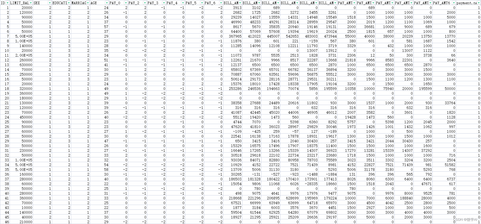
数据样例：

二、数据分析和可视化

1.查看年龄分布情况

# 查看年龄分布情况
age = data['AGE']
payment = data[data["payment.next.month"]==1]['AGE']
bins =[20,30,40,50,60,70,80]
seg = pd.cut(age,bins,right=False)
print(seg)
counts =pd.value_counts(seg,sort=False)
b = plt.bar(counts.index.astype(str),counts)
plt.bar_label(b,counts)
plt.show()

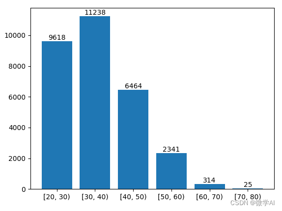
信用卡使用最多的年龄是在30-40岁之间，有11238人，其实是20-30岁的人，有9618人，80后90后是信用卡使用的大军。
信用卡有逾期的客户年龄分布：

#逾期的用户年龄分布
payment_seg = pd.cut(payment,bins,right=False)
counts1 =pd.value_counts(payment_seg,sort=False)
b2 = plt.bar(counts1.index.astype(str),counts1,color='r')
plt.bar_label(b2,counts1)
plt.show()

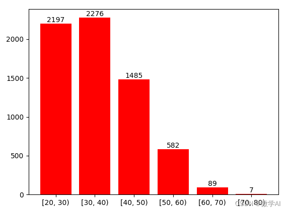
逾期率对比：
20-30岁：22.84%，
30-40岁：20.25%，
40-50岁：22.97，
50-60岁：24.86%，
70-80岁：28%
可以看出70-80岁逾期率最高，可能是他们年龄的原因忘记还款，或者子女未帮忙还款所致；

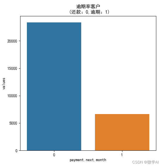
2.查看下一个月逾期率的情况

next_month = data['payment.next.month'].value_counts()
print(next_month)
df = pd.DataFrame({'payment.next.month': next_month.index,'values': next_month.values})
plt.rcParams['font.sans-serif']=['SimHei'] #用来正常显示中文标签
plt.figure(figsize = (6,6))

plt.title('逾期率客户\n (还款：0,逾期：1)')
sns.set_color_codes("pastel")
sns.barplot(x = 'payment.next.month', y="values", data=df)
plt.show()

三、数据特征处理

# 特征选择，去掉ID字段、最后一个结果字段即可
data.drop(['ID'], inplace=True, axis =1) #ID这个字段没有用
target = data['payment.next.month'].values
columns = data.columns.tolist()
columns.remove('payment.next.month')
features = data[columns].values

# 70%作为训练集，30%作为测试集
train_x, test_x, train_y, test_y = train_test_split(features, target, test_size=0.30, stratify = target, random_state = 1)

四、机器学习算法分类器

下面我们采用四种机器学习算法进行分类预测，分别是支持向量机、决策树、随机森林、 K近邻算法，小伙伴是不是对这四类算法一下子有了熟悉的感觉。

# 构造各种分类器
classifiers = [
    SVC(random_state = 1, kernel = 'rbf'),     # 支持向量机分类
    DecisionTreeClassifier(random_state = 1, criterion = 'gini'),  # 决策树分类
    RandomForestClassifier(random_state = 1, criterion = 'gini'),  # 随机森林分类
    KNeighborsClassifier(metric = 'minkowski'),    # K近邻分类
]
# 分类器名称
classifier_names = [
            'svc',
            'decisiontreeclassifier',
            'randomforestclassifier',
            'kneighborsclassifier',
]
# 分类器参数
classifier_param_grid = [
            {'svc__C':[1], 'svc__gamma':[0.01]},
            {'decisiontreeclassifier__max_depth':[6,9,11]},
            {'randomforestclassifier__n_estimators':[3,5,6]} ,
            {'kneighborsclassifier__n_neighbors':[4,6,8]},
]

五、参数调优

# 对具体的分类器进行GridSearchCV参数调优
def GridSearchCV_work(pipeline, train_x, train_y, test_x, test_y, param_grid, score = 'accuracy'):
    response = {}
    gridsearch = GridSearchCV(estimator = pipeline, param_grid = param_grid, scoring = score)

    # 寻找最优的参数 和最优的准确率分数
    search = gridsearch.fit(train_x, train_y)
    print("GridSearch最优参数：", search.best_params_)
    print("GridSearch最优分数： %0.4lf" %search.best_score_)
    predict_y = gridsearch.predict(test_x)
    print("准确率 %0.4lf" %accuracy_score(test_y, predict_y))
    response['predict_y'] = predict_y
    response['accuracy_score'] = accuracy_score(test_y,predict_y)
    return response

六、模型对比分析

for model, model_name, model_param_grid in zip(classifiers, classifier_names, classifier_param_grid):
    pipeline = Pipeline([
            ('scaler', StandardScaler()),
            (model_name, model)
    ])
    result = GridSearchCV_work(pipeline, train_x, train_y, test_x, test_y, model_param_grid , score = 'accuracy')

Name: payment.next.month, dtype: int64
GridSearch最优参数： {'svc__C': 1, 'svc__gamma': 0.01}
GridSearch最优分数： 0.8186
准确率 0.8172
GridSearch最优参数： {'decisiontreeclassifier__max_depth': 6}
GridSearch最优分数： 0.8208
准确率 0.8113
GridSearch最优参数： {'randomforestclassifier__n_estimators': 6}
GridSearch最优分数： 0.8004
准确率 0.7994
GridSearch最优参数： {'kneighborsclassifier__n_neighbors': 8}
GridSearch最优分数： 0.8040
准确率 0.8036

我们可以看到运行结果：
支持向量机算法分类：准确率 0.8172
决策树算法分类：准确率 0.8113
随机森林分类：准确率 0.7994
K近邻分类：准确率 0.8036
这四种算法中，准确率都差不多，其中准确率最高的是支持向量机算法。
数据集的获取，可以私信我，更多精彩的实战内容，后期将献给大家，谢谢。