科技主题基金数据分析

科技基金数据分析

1. 基金的收益分布分析

2. 建立风险测度模型

一、数据预处理

#设置工作路径
setwd("D:/LengPY")

#导入数据
library(readxl)
lqydata<-read_excel("lqydata.xlsx")

head(lqydata)

A tibble: 6 × 25

基金代码	基金名称	投资类型	类别	成立时间	基金经理累计从业时间	基金净值	基金规模	阿尔法系数	贝塔系数	...	近一周	近一月	近三月	近六月	今年来	近一年	近两年	近三年	晨星风险系数	风险评级
<chr>	<chr>	<chr>	<chr>	<dbl>	<dbl>	<chr>	<dbl>	<dbl>	<dbl>	...	<dbl>	<dbl>	<dbl>	<dbl>	<dbl>	<dbl>	<dbl>	<dbl>	<dbl>	<chr>
000209	信诚新兴产业混合	混合型	新能源	2013	6	2.9870	4.11	16.04	1.15	...	8.30	13.23	-12.02	42.51	3.25	107.57	143.24	117.24	16.51	中
000336	农银研究精选混合	混合型	新能源	2013	4	3.5356	30.43	27.36	1.16	...	4.61	6.57	-13.89	24.72	-3.66	119.62	203.30	183.60	14.44	中
000409	鹏华环保产业股票	股票型	新能源	2014	3	3.8880	13.87	20.73	0.98	...	5.80	9.92	-15.97	21.01	-6.74	87.01	134.78	141.19	12.56	中高
000432	中银优秀企业混合	混合型	人工智能	2014	3	2.1320	0.23	4.33	0.79	...	3.29	5.70	-6.20	-2.60	-5.29	11.22	31.85	44.35	10.35	中高
000432	中银优秀企业混合	混合型	国产软件	2014	3	2.1320	0.23	4.33	0.79	...	3.29	5.70	-6.20	-2.60	-5.29	11.22	31.85	44.35	10.35	中高
000535	长盛航天海工装备	混合型	无人机	2014	5	1.3400	3.16	4.98	0.97	...	-0.52	-0.96	-20.94	1.43	-18.38	39.71	40.87	43.69	11.05	中

summary(lqydata)

   基金代码           基金名称           投资类型             类别          
 Length:102         Length:102         Length:102         Length:102        
 Class :character   Class :character   Class :character   Class :character  
 Mode  :character   Mode  :character   Mode  :character   Mode  :character  
                                                                            
                                                                            
                                                                            
    成立时间    基金经理累计从业时间   基金净值            基金规模      
 Min.   :2003   Min.   : 1.000       Length:102         Min.   :  0.090  
 1st Qu.:2014   1st Qu.: 3.000       Class :character   1st Qu.:  2.505  
 Median :2015   Median : 5.000       Mode  :character   Median :  5.035  
 Mean   :2014   Mean   : 4.941                          Mean   : 19.211  
 3rd Qu.:2016   3rd Qu.: 6.000                          3rd Qu.: 12.797  
 Max.   :2018   Max.   :11.000                          Max.   :271.100  
   阿尔法系数         贝塔系数          R平方           标准差     
 Min.   :-10.100   Min.   :0.7100   Min.   : 4.79   Min.   :18.22  
 1st Qu.:  1.627   1st Qu.:0.8525   1st Qu.:59.33   1st Qu.:25.27  
 Median :  5.385   Median :0.9700   Median :75.25   Median :27.25  
 Mean   :  6.947   Mean   :1.0204   Mean   :73.52   Mean   :27.20  
 3rd Qu.: 12.002   3rd Qu.:1.1300   3rd Qu.:92.53   3rd Qu.:29.52  
 Max.   : 27.360   Max.   :2.8200   Max.   :99.20   Max.   :36.01  
    夏普比率          回报率          日增长率           近一周      
 Min.   :-0.110   Min.   : -9.42   Min.   :-1.1900   Min.   :-1.190  
 1st Qu.: 0.320   1st Qu.: 15.38   1st Qu.:-0.2775   1st Qu.: 2.170  
 Median : 0.450   Median : 29.96   Median : 0.2800   Median : 3.370  
 Mean   : 0.515   Mean   : 37.73   Mean   : 0.3211   Mean   : 3.601  
 3rd Qu.: 0.715   3rd Qu.: 57.66   3rd Qu.: 0.9500   3rd Qu.: 5.420  
 Max.   : 1.200   Max.   :117.37   Max.   : 1.8400   Max.   : 8.960  
     近一月           近三月            近六月            今年来       
 Min.   :-2.250   Min.   :-25.090   Min.   :-13.900   Min.   :-22.130  
 1st Qu.: 4.940   1st Qu.:-15.625   1st Qu.: -1.275   1st Qu.: -6.885  
 Median : 6.755   Median :-11.435   Median :  4.265   Median : -4.125  
 Mean   : 6.610   Mean   :-12.630   Mean   :  7.434   Mean   : -5.142  
 3rd Qu.: 8.910   3rd Qu.: -9.592   3rd Qu.: 16.517   3rd Qu.: -1.090  
 Max.   :15.560   Max.   : -5.060   Max.   : 42.510   Max.   :  7.340  
     近一年           近两年           近三年        晨星风险系数  
 Min.   :-11.74   Min.   : -1.31   Min.   : -4.18   Min.   :10.35  
 1st Qu.: 15.41   1st Qu.: 41.02   1st Qu.: 30.46   1st Qu.:13.78  
 Median : 29.32   Median : 53.62   Median : 47.91   Median :15.21  
 Mean   : 36.85   Mean   : 64.63   Mean   : 61.63   Mean   :15.55  
 3rd Qu.: 54.02   3rd Qu.: 87.98   3rd Qu.: 86.92   3rd Qu.:16.20  
 Max.   :119.62   Max.   :203.30   Max.   :183.60   Max.   :31.01  
   风险评级        
 Length:102        
 Class :character  
 Mode  :character  

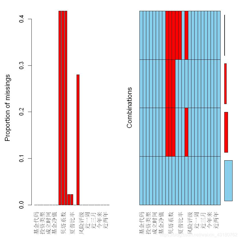
#检查是否有缺失值
## 可视化查看数据是否有缺失值
library(VIM)
aggr(lqydata)

## complete.cases()输出样例是否包含缺失值
## 输出包含缺失值的样例
mynadata <- lqydata[!complete.cases(lqydata),]
dim(mynadata)

1. 0
2. 25

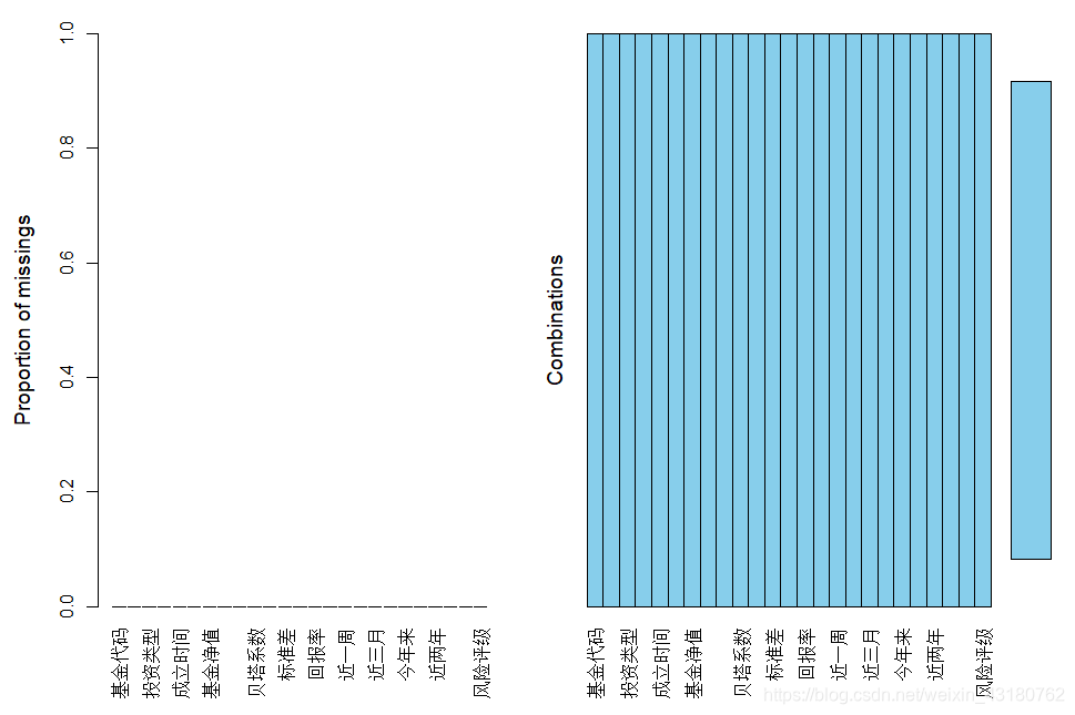
## matrixplot()可视化缺失值的详细情况
## 红色代表缺失数据的情况
matrixplot(mynadata)  

分析可知，是由于新成立基金公司缺失值验证，可直接删除对应样本可得：

head(lqydata)

A tibble: 6 × 25

基金代码	基金名称	投资类型	类别	成立时间	基金经理累计从业时间	基金净值	基金规模	阿尔法系数	贝塔系数	...	近一周	近一月	近三月	近六月	今年来	近一年	近两年	近三年	晨星风险系数	风险评级
<chr>	<chr>	<chr>	<chr>	<dbl>	<dbl>	<chr>	<dbl>	<dbl>	<dbl>	...	<dbl>	<dbl>	<dbl>	<dbl>	<dbl>	<dbl>	<dbl>	<dbl>	<dbl>	<chr>
000209	信诚新兴产业混合	混合型	新能源	2013	6	2.9870	4.11	16.04	1.15	...	8.30	13.23	-12.02	42.51	3.25	107.57	143.24	117.24	16.51	中
000336	农银研究精选混合	混合型	新能源	2013	4	3.5356	30.43	27.36	1.16	...	4.61	6.57	-13.89	24.72	-3.66	119.62	203.30	183.60	14.44	中
000409	鹏华环保产业股票	股票型	新能源	2014	3	3.8880	13.87	20.73	0.98	...	5.80	9.92	-15.97	21.01	-6.74	87.01	134.78	141.19	12.56	中高
000432	中银优秀企业混合	混合型	人工智能	2014	3	2.1320	0.23	4.33	0.79	...	3.29	5.70	-6.20	-2.60	-5.29	11.22	31.85	44.35	10.35	中高
000432	中银优秀企业混合	混合型	国产软件	2014	3	2.1320	0.23	4.33	0.79	...	3.29	5.70	-6.20	-2.60	-5.29	11.22	31.85	44.35	10.35	中高
000535	长盛航天海工装备	混合型	无人机	2014	5	1.3400	3.16	4.98	0.97	...	-0.52	-0.96	-20.94	1.43	-18.38	39.71	40.87	43.69	11.05	中

二、基础分布描述性分析

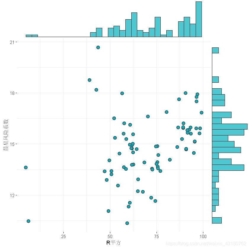
2.1 R平方与风险系数散点分布图

#(a) 二维散点与统计直方图
library(ggplot2)
library(RColorBrewer)
library(ggpubr)
ggscatterhist(
  lqydata, x ='R平方', y = '晨星风险系数', shape=21,fill="#00AFBB",color = "black",size = 3, alpha = 1,
  #palette = c("#00AFBB", "#E7B800", "#FC4E07"),
  margin.params = list( fill="#00AFBB",color = "black", size = 0.2,alpha=1),
  margin.plot =  "histogram",
  legend = c(0.8,0.8),
  ggtheme = theme_minimal())

table(lqydata$类别)

  半导体 国产软件 国产芯片 人工智能 生物识别   无人机   新能源 智能穿戴 
       6       24        7       13        7       14       24        7 

data1<-as.data.frame(table(lqydata$类别))
colnames(data1)<-c('type','num')
head(data1)

A data.frame: 6 × 2

	type	num
	<fct>	<int>
1	半导体	6
2	国产软件	24
3	国产芯片	7
4	人工智能	13
5	生物识别	7
6	无人机	14

#"半导体","国产软件","国产芯片","人工智能","生物识别","无人机"
#16,37,16,17,16,22

table(lqydata$成立时间)

2003 2004 2006 2007 2009 2010 2011 2012 2013 2014 2015 2016 2017 2018 
   2    1    1    1    2    5    7    1    2   20   32    8   17    3 

table(lqydata$投资类型)

  股票型 股票指数   混合型 联接基金 
      22       33       30       17 

lqydata$基金净值<-as.numeric( lqydata$基金净值) 

3.2 探索相关性

colnames(lqydata)

1. '基金代码'
2. '基金名称'
3. '投资类型'
4. '类别'
5. '成立时间'
6. '基金经理累计从业时间'
7. '基金净值'
8. '基金规模'
9. '阿尔法系数'
10. '贝塔系数'
11. 'R平方'
12. '标准差'
13. '夏普比率'
14. '回报率'
15. '日增长率'
16. '近一周'
17. '近一月'
18. '近三月'
19. '近六月'
20. '今年来'
21. '近一年'
22. '近两年'
23. '近三年'
24. '晨星风险系数'
25. '风险评级'

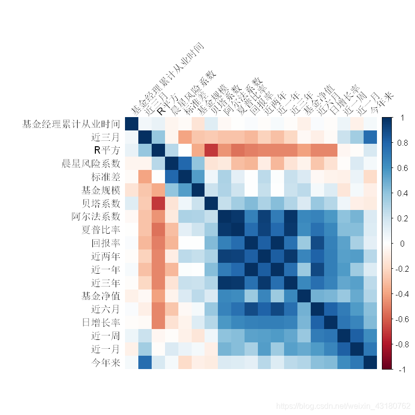
mcor<-cor(lqydata[,c(6:24)])
library(corrplot) # 载入corrplot包
corrplot(mcor)

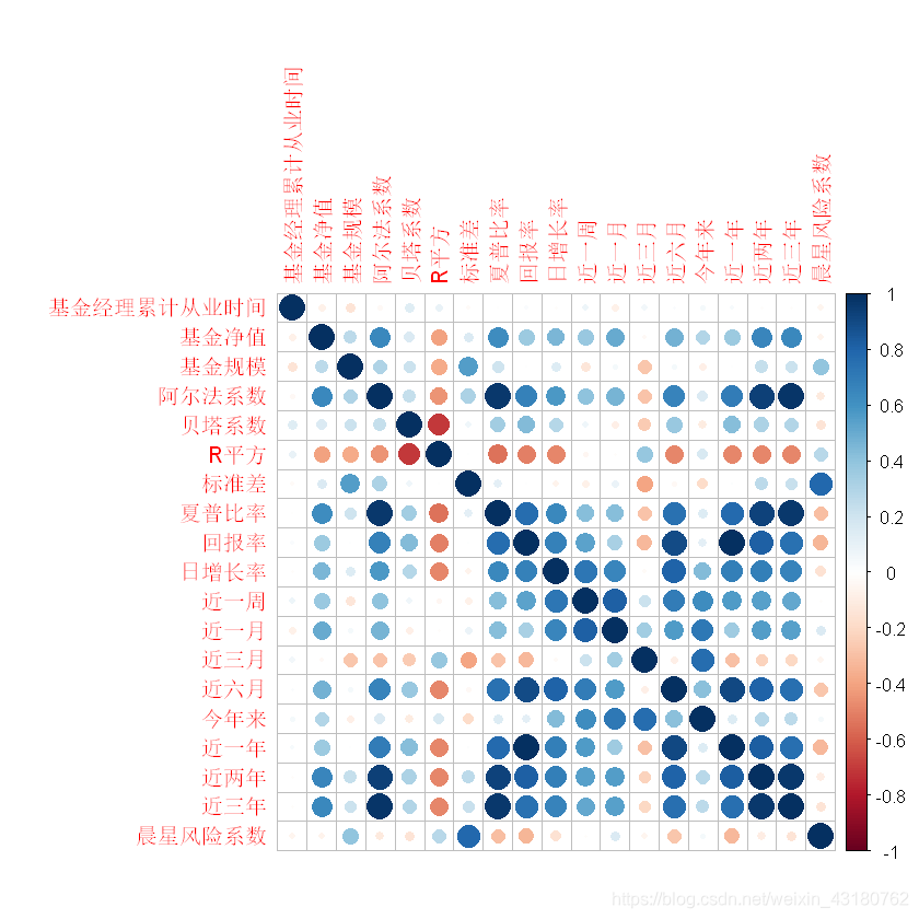
corrplot(mcor, method = "shade",shade.col = NA, tl.col ="black", tl.srt = 45, order = "AOE") # 绘制相关系数矩阵图

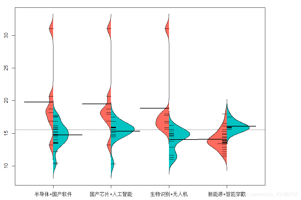
三、探索基金收益分布之间规律及其分布情况

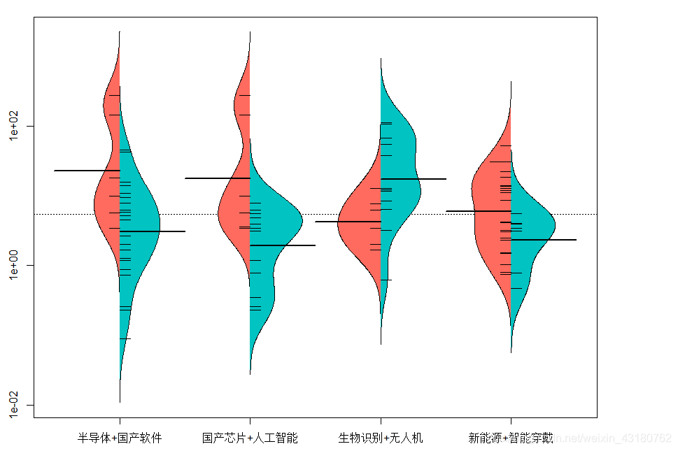
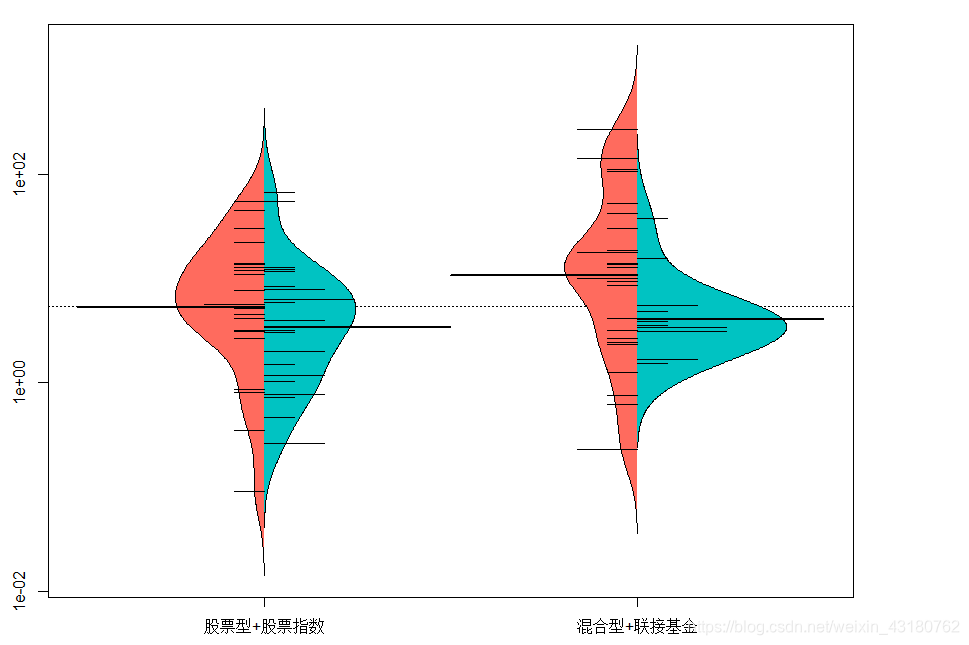
3.1 不同主题基金规模分布对比

#转换为数值型
lqydata$基金规模<-as.numeric(lqydata$基金规模)

#不同主题基金规模之间对比
library(beanplot)
par(mai=c(0.5,0.5,0.25,1.2))
beanplot(基金规模~类别, lqydata,col = list("#FF6B5E", "#00C3C2"),
         side = "both",xlab ="city",ylab ="value")

Warning message:
"package 'beanplot' was built under R version 4.0.5"
log="y" selected

3.2 不同主题基金回报率分布

#回报率（一年）
#不同主题之间对比
library(beanplot)
par(mai=c(0.5,0.5,0.25,1.2))
beanplot(lqydata$回报率~lqydata$类别, lqydata,col = list("#FF6B5E", "#00C3C2"),
         side = "both",xlab ="city",ylab ="value")

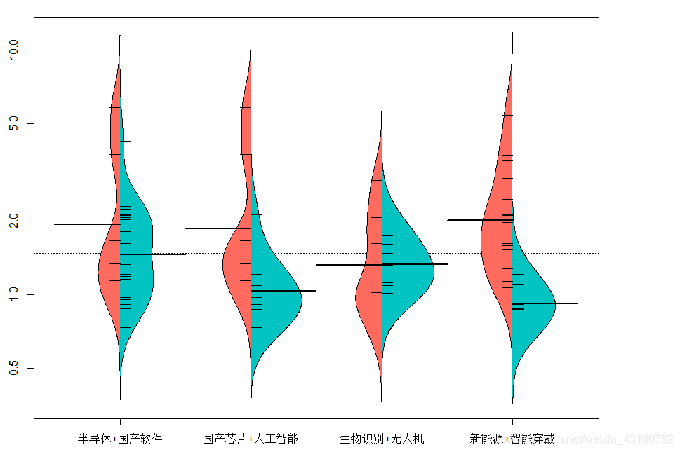
3.3不同主题基金净值之间对比

#不同主题之间对比
library(beanplot)
par(mai=c(0.5,0.5,0.25,1.2))
beanplot(lqydata$基金净值~lqydata$类别, lqydata,col = list("#FF6B5E", "#00C3C2"),
         side = "both",xlab ="city",ylab ="value")

log="y" selected

colnames(lqydata)

1. '基金代码'
2. '基金名称'
3. '投资类型'
4. '类别'
5. '成立时间'
6. '基金经理累计从业时间'
7. '基金净值'
8. '基金规模'
9. '阿尔法系数（%）'
10. '贝塔系数'
11. 'R平方'
12. '标准差（%）'
13. '夏普比率'
14. '回报率'
15. '日增长率'
16. '近一周'
17. '近一月'
18. '近三月'
19. '近六月'
20. '今年来'
21. '近一年'
22. '近两年'
23. '近三年'
24. '晨星风险系数'
25. '风险评级'

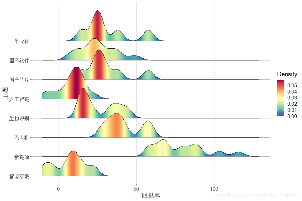
3.4 不同主题基金回报率分布

#一年回报率
library(reshape2)
library(ggplot2)
library(ggridges)
library(RColorBrewer)
colormap <- colorRampPalette(rev(brewer.pal(11,'Spectral')))(32)
dt<-lqydata[,c(4,14)]
colnames(dt)<-c("主题","收益率")
splitdata<-split(dt,dt$主题)
xmax<-max(dt$`收益率`)*1.1
xmin<-min(dt$`收益率`)*1.1


N<-length(splitdata)
labels_y<-names(splitdata)

mydata<-data.frame(x=numeric(),y=numeric(),variable=numeric()) #?????յ?Data.Frame

for (i in 1:N){
  tempy<-density(splitdata[[i]][2]$`收益率`,bw = 3.37,from=xmin, to=xmax)
  newdata<-data.frame(x=tempy$x,y=tempy$y)
  newdata$variable<-i
  mydata<-rbind(mydata,newdata)
}

Step<-max(mydata$y)*0.6
mydata$offest<--as.numeric(mydata$variable)*Step
mydata$V1_density_offest<-mydata$y+mydata$offest

p<-ggplot()
for (i in 1:N){
  p<-p+ geom_linerange(data=mydata[mydata$variable==i,],aes(x=x,ymin=offest,ymax=V1_density_offest,group=variable,color=y),size =1, alpha =1) +
        geom_line(data=mydata[mydata$variable==i,],aes(x=x, y=V1_density_offest),color="black",size=0.5)
}

p+scale_color_gradientn(colours=colormap,name="Density")+
  scale_y_continuous(breaks=seq(-Step,-Step*N,-Step),labels=labels_y)+
  xlab("回报率")+
  ylab("主题")+
  theme_classic()+
  theme(
    panel.background=element_rect(fill="white",colour=NA),
    panel.grid.major.x = element_line(colour = "grey80",size=.25),
    panel.grid.major.y = element_line(colour = "grey60",size=.25),
    axis.line = element_blank(),
    text=element_text(size=15,colour = "black"),
    plot.title=element_text(size=15,hjust=.5),
    legend.position="right"
  )

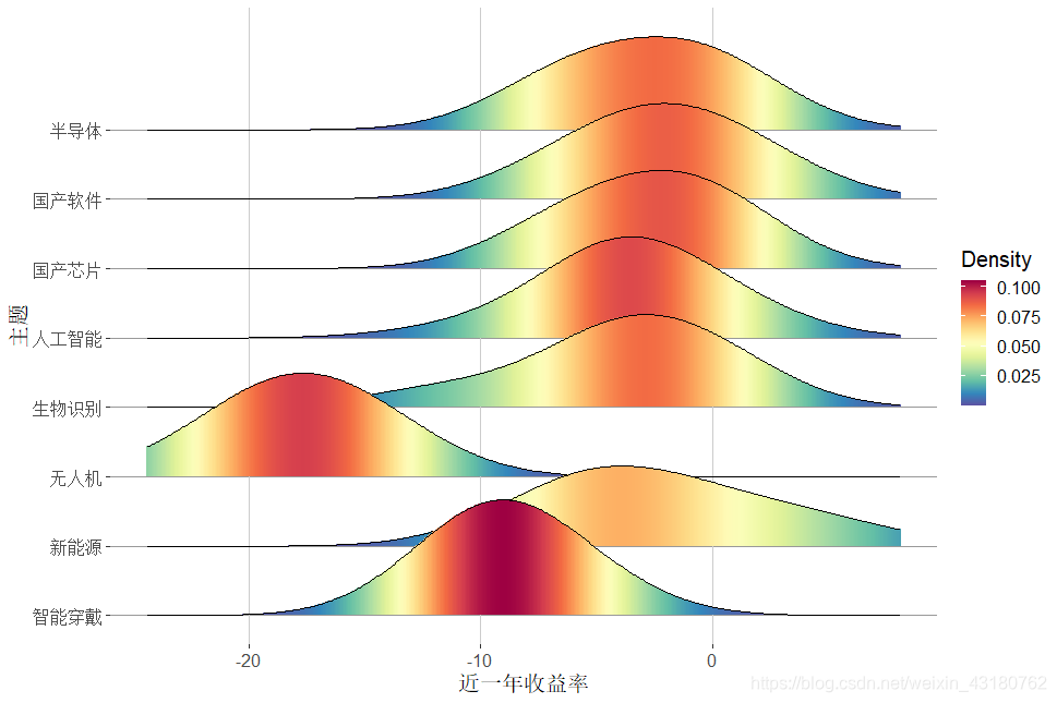
3.5 近一年增长率分布情况

#近一年收益率分布情况
library(reshape2)
library(ggplot2)
library(ggridges)
library(RColorBrewer)
colormap <- colorRampPalette(rev(brewer.pal(11,'Spectral')))(32)
dt<-lqydata[,c(4,20)]
colnames(dt)<-c("主题","收益率")
splitdata<-split(dt,dt$主题)
xmax<-max(dt$`收益率`)*1.1
xmin<-min(dt$`收益率`)*1.1


N<-length(splitdata)
labels_y<-names(splitdata)

mydata<-data.frame(x=numeric(),y=numeric(),variable=numeric()) #?????յ?Data.Frame

for (i in 1:N){
  tempy<-density(splitdata[[i]][2]$`收益率`,bw = 3.37,from=xmin, to=xmax)
  newdata<-data.frame(x=tempy$x,y=tempy$y)
  newdata$variable<-i
  mydata<-rbind(mydata,newdata)
}

Step<-max(mydata$y)*0.6
mydata$offest<--as.numeric(mydata$variable)*Step
mydata$V1_density_offest<-mydata$y+mydata$offest

p<-ggplot()
for (i in 1:N){
  p<-p+ geom_linerange(data=mydata[mydata$variable==i,],aes(x=x,ymin=offest,ymax=V1_density_offest,group=variable,color=y),size =1, alpha =1) +
        geom_line(data=mydata[mydata$variable==i,],aes(x=x, y=V1_density_offest),color="black",size=0.5)
}

p+scale_color_gradientn(colours=colormap,name="Density")+
  scale_y_continuous(breaks=seq(-Step,-Step*N,-Step),labels=labels_y)+
  xlab("近一年收益率")+
  ylab("主题")+
  theme_classic()+
  theme(
    panel.background=element_rect(fill="white",colour=NA),
    panel.grid.major.x = element_line(colour = "grey80",size=.25),
    panel.grid.major.y = element_line(colour = "grey60",size=.25),
    axis.line = element_blank(),
    text=element_text(size=15,colour = "black"),
    plot.title=element_text(size=15,hjust=.5),
    legend.position="right"
  )

3.8 不同投资类型的基金规模情况

library(beanplot)
par(mai=c(0.5,0.5,0.25,1.2))
beanplot(基金规模~投资类型, lqydata,col = list("#FF6B5E", "#00C3C2"),
         side = "both",xlab ="city",ylab ="value")

log="y" selected

3.9 基金规模分布情况

hist(lqydata$基金规模, prob = TRUE, col = "lightblue",main="Normal Distribution") 

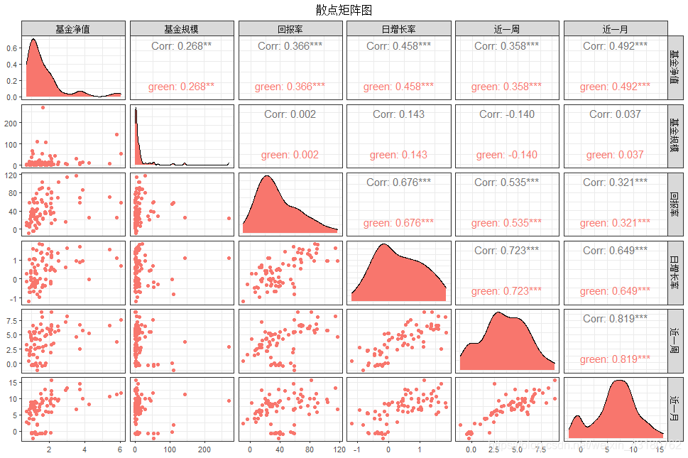
3.12 收益矩阵分布图

#基金收益矩阵图
lqy<-lqydata[,c(7,8,14:23)]
library(GGally) 
ggpairs(lqy,columns=c(1:6),aes(color='green'),alpha=0.8)+ 
 theme_bw(base_family="STKaiti",base_size=10)+ 
 theme(plot.title=element_text(hjust=0.5))+ 
 ggtitle("散点矩阵图")

四、基金风险分布可视化

4.1 不同主题晨星风险系数之间对比

#不同主题之间对比
library(beanplot)
par(mai=c(0.5,0.5,0.25,1.2))
beanplot(晨星风险系数~类别, lqydata,col = list("#FF6B5E", "#00C3C2"),
         side = "both",xlab ="city",ylab ="value")

4.2 风险分布矩阵图，验证风险评级是否能区分开数据

#风险分布矩阵图
lqy<-lqydata[,c(9:13,24,25)]
library(GGally) 
ggpairs(lqy,columns=c(1:6),aes(color=风险评级),alpha=0.8)+ 
 theme_bw(base_family="STKaiti",base_size=10)+ 
 theme(plot.title=element_text(hjust=0.5))+ 
 ggtitle("散点矩阵图")

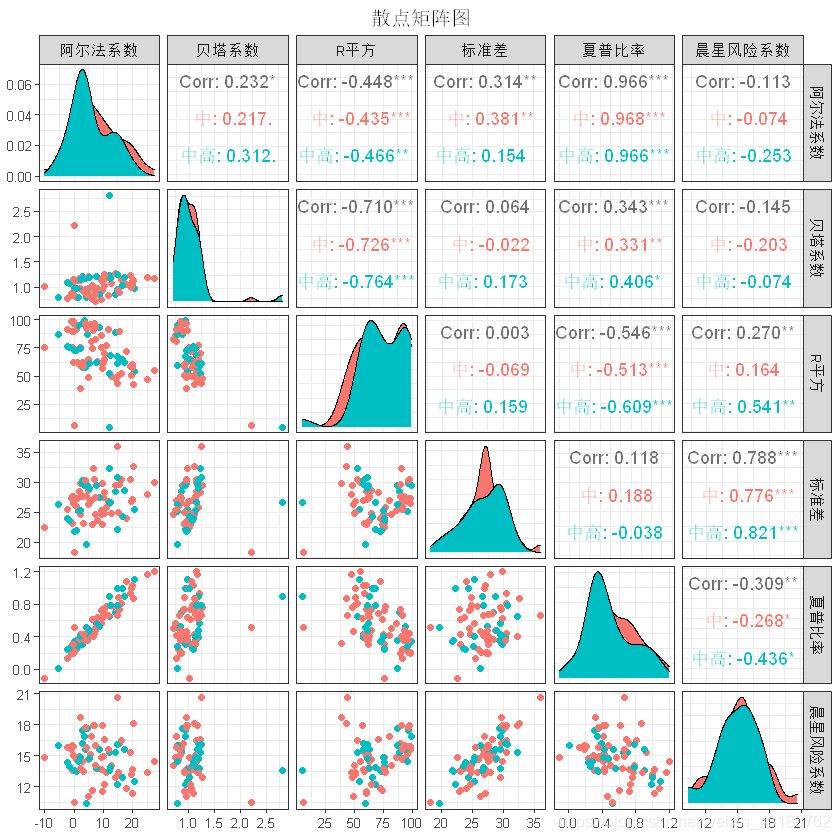
数据中原给定的风险评级，并未能将各风险指标区分开，故该风险评级存在一定的局限性，设法改进。

聚类结果较不理想，考虑更换风险度量指标后再进行聚类。

4.3 基金风险聚类评估

colnames(lqydata)

1. '基金代码'
2. '基金名称'
3. '投资类型'
4. '类别'
5. '成立时间'
6. '基金经理累计从业时间'
7. '基金净值'
8. '基金规模'
9. '阿尔法系数（%）'
10. '贝塔系数'
11. 'R平方'
12. '标准差（%）'
13. '夏普比率'
14. '回报率'
15. '日增长率'
16. '近一周'
17. '近一月'
18. '近三月'
19. '近六月'
20. '今年来'
21. '近一年'
22. '近两年'
23. '近三年'
24. '晨星风险系数'
25. '风险评级'

cludata<-lqydata[,c(1,2,9:13,24)]

head(cludata)

A tibble: 6 × 8

基金代码	基金名称	阿尔法系数（%）	贝塔系数	R平方	标准差（%）	夏普比率	晨星风险系数
<chr>	<chr>	<dbl>	<dbl>	<dbl>	<dbl>	<dbl>	<dbl>
000209	信诚新兴产业混合	16.04	1.15	52.20	30.49	0.81	16.51
000336	农银研究精选混合	27.36	1.16	55.08	29.87	1.20	14.44
000409	鹏华环保产业股票	20.73	0.98	54.30	25.37	1.10	12.56
000432	中银优秀企业混合	4.33	0.79	59.33	19.62	0.52	10.35
000432	中银优秀企业混合	4.33	0.79	59.33	19.62	0.52	10.35
000535	长盛航天海工装备	4.98	0.97	49.26	26.32	0.46	11.05

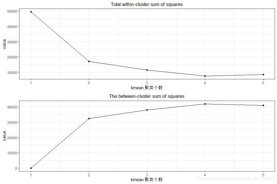
## 计算组内平方和  组间平方和
tot_withinss <- vector()
betweenss <- vector()
for(ii in 1:5){
  k1 <- kmeans(cludata[,c(3:7)],ii)
  tot_withinss[ii] <- k1$tot.withinss
  betweenss[ii] <- k1$betweenss
}

kmeanvalue <- data.frame(kk = 1:5,
                         tot_withinss = tot_withinss,
                         betweenss = betweenss)

library(ggplot2)
library(gridExtra)
library(ggdendro)
library(cluster)
library(ggfortify)
p1 <- ggplot(kmeanvalue,aes(x = kk,y = tot_withinss))+
  theme_bw()+
  geom_point() + geom_line() +labs(y = "value") +
  ggtitle("Total within-cluster sum of squares")+
  theme(plot.title = element_text(hjust = 0.5))+
  scale_x_continuous("kmean 聚类个数",kmeanvalue$kk)

p2 <- ggplot(kmeanvalue,aes(x = kk,y = betweenss))+
  theme_bw()+
  geom_point() +geom_line() +labs(y = "value") +
  ggtitle("The between-cluster sum of squares") +
  theme(plot.title = element_text(hjust = 0.5))+
  scale_x_continuous("kmean 聚类个数",kmeanvalue$kk)

grid.arrange(p1,p2,nrow=2)

Warning message:
"package 'ggplot2' was built under R version 4.0.4"
Warning message:
"package 'gridExtra' was built under R version 4.0.4"
Warning message:
"package 'ggdendro' was built under R version 4.0.4"
Warning message:
"package 'ggfortify' was built under R version 4.0.4"

set.seed(245)
k3 <- kmeans(cludata[,c(3:7)],2)
summary(k3)

             Length Class  Mode   
cluster      102    -none- numeric
centers       10    -none- numeric
totss          1    -none- numeric
withinss       2    -none- numeric
tot.withinss   1    -none- numeric
betweenss      1    -none- numeric
size           2    -none- numeric
iter           1    -none- numeric
ifault         1    -none- numeric

#将标签写入
cludata$cluster<-k3$cluster
head(cludata)
cludata$cluster<-as.factor(cludata$cluster)

A tibble: 6 × 9

基金代码	基金名称	阿尔法系数（%）	贝塔系数	R平方	标准差（%）	夏普比率	晨星风险系数	cluster
<chr>	<chr>	<dbl>	<dbl>	<dbl>	<dbl>	<dbl>	<dbl>	<int>
000209	信诚新兴产业混合	16.04	1.15	52.20	30.49	0.81	16.51	2
000336	农银研究精选混合	27.36	1.16	55.08	29.87	1.20	14.44	2
000409	鹏华环保产业股票	20.73	0.98	54.30	25.37	1.10	12.56	2
000432	中银优秀企业混合	4.33	0.79	59.33	19.62	0.52	10.35	2
000432	中银优秀企业混合	4.33	0.79	59.33	19.62	0.52	10.35	2
000535	长盛航天海工装备	4.98	0.97	49.26	26.32	0.46	11.05	2

#基金收益矩阵图
library(GGally) 
ggpairs(cludata[,3:9],columns=c(1:6),aes(color=cluster),alpha=0.8)+ 
 theme_bw(base_family="STKaiti",base_size=10)+ 
 theme(plot.title=element_text(hjust=0.5))+ 
 ggtitle("散点矩阵图")

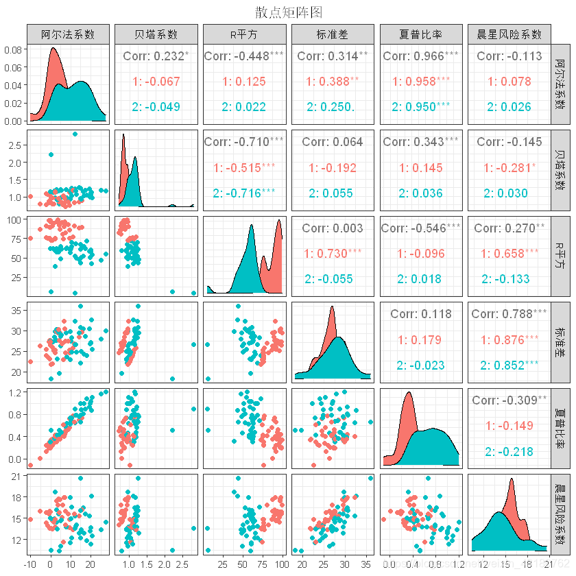
聚类为2类时，数据区分度较高，模型合理

## 对聚类结果可视化
clusplot(cludata[,c(3:7)],k3$cluster,main = "kmean cluster number=2")

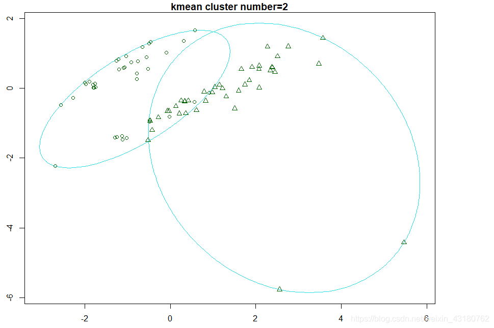
#如果分为三类
set.seed(245)
k3 <- kmeans(cludata[,c(3:7)],3)
summary(k3)

             Length Class  Mode   
cluster      102    -none- numeric
centers       15    -none- numeric
totss          1    -none- numeric
withinss       3    -none- numeric
tot.withinss   1    -none- numeric
betweenss      1    -none- numeric
size           3    -none- numeric
iter           1    -none- numeric
ifault         1    -none- numeric

#将标签写入
cludata$cluster<-k3$cluster
head(cludata)
cludata$cluster<-as.factor(cludata$cluster)

A tibble: 6 × 9

基金代码	基金名称	阿尔法系数（%）	贝塔系数	R平方	标准差（%）	夏普比率	晨星风险系数	cluster
<chr>	<chr>	<dbl>	<dbl>	<dbl>	<dbl>	<dbl>	<dbl>	<int>
000209	信诚新兴产业混合	16.04	1.15	52.20	30.49	0.81	16.51	2
000336	农银研究精选混合	27.36	1.16	55.08	29.87	1.20	14.44	2
000409	鹏华环保产业股票	20.73	0.98	54.30	25.37	1.10	12.56	2
000432	中银优秀企业混合	4.33	0.79	59.33	19.62	0.52	10.35	2
000432	中银优秀企业混合	4.33	0.79	59.33	19.62	0.52	10.35	2
000535	长盛航天海工装备	4.98	0.97	49.26	26.32	0.46	11.05	2

## 对聚类结果可视化
clusplot(cludata[,c(3:7)],k3$cluster,main = "kmean cluster number=3")

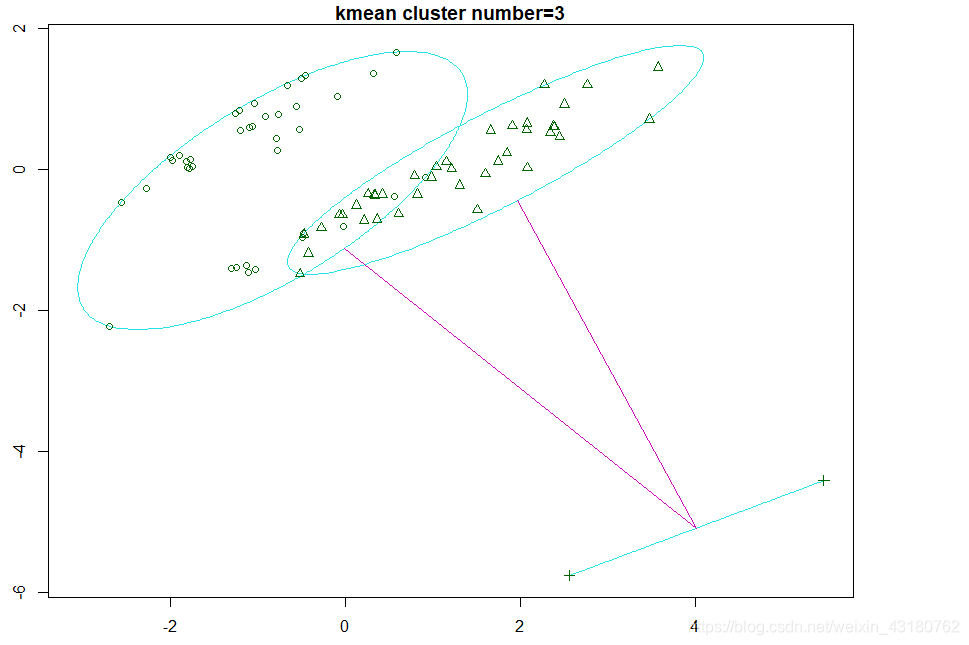
此时模型得到合适的分类，比较合理

可知，分为2-3类也较合理

五、建立风险评估模型

5.1 选取建模指标

colnames(lqydata)

1. '基金代码'
2. '基金名称'
3. '投资类型'
4. '类别'
5. '成立时间'
6. '基金经理累计从业时间'
7. '基金净值'
8. '基金规模'
9. '阿尔法系数'
10. '贝塔系数'
11. 'R平方'
12. '标准差'
13. '夏普比率'
14. '回报率'
15. '日增长率'
16. '近一周'
17. '近一月'
18. '近三月'
19. '近六月'
20. '今年来'
21. '近一年'
22. '近两年'
23. '近三年'
24. '晨星风险系数'
25. '风险评级'

#由于风险评级并不能有效地区分开样本，故可暂时进行剔除
scoredata<-lqydata[,c(-1,-2,-25)]
head(scoredata)

A tibble: 6 × 22

投资类型	类别	成立时间	基金经理累计从业时间	基金净值	基金规模	阿尔法系数	贝塔系数	R平方	标准差	...	日增长率	近一周	近一月	近三月	近六月	今年来	近一年	近两年	近三年	晨星风险系数
<chr>	<chr>	<dbl>	<dbl>	<dbl>	<dbl>	<dbl>	<dbl>	<dbl>	<dbl>	...	<dbl>	<dbl>	<dbl>	<dbl>	<dbl>	<dbl>	<dbl>	<dbl>	<dbl>	<dbl>
混合型	新能源	2013	6	2.9870	4.11	16.04	1.15	52.20	30.49	...	1.60	8.30	13.23	-12.02	42.51	3.25	107.57	143.24	117.24	16.51
混合型	新能源	2013	4	3.5356	30.43	27.36	1.16	55.08	29.87	...	0.95	4.61	6.57	-13.89	24.72	-3.66	119.62	203.30	183.60	14.44
股票型	新能源	2014	3	3.8880	13.87	20.73	0.98	54.30	25.37	...	0.96	5.80	9.92	-15.97	21.01	-6.74	87.01	134.78	141.19	12.56
混合型	人工智能	2014	3	2.1320	0.23	4.33	0.79	59.33	19.62	...	0.61	3.29	5.70	-6.20	-2.60	-5.29	11.22	31.85	44.35	10.35
混合型	国产软件	2014	3	2.1320	0.23	4.33	0.79	59.33	19.62	...	0.61	3.29	5.70	-6.20	-2.60	-5.29	11.22	31.85	44.35	10.35
混合型	无人机	2014	5	1.3400	3.16	4.98	0.97	49.26	26.32	...	-0.22	-0.52	-0.96	-20.94	1.43	-18.38	39.71	40.87	43.69	11.05

5.2 建立支持向量机模型

## 支持向量机回归模型
library(e1071)
library(caret)
library(Metrics)
library(readr)

system.time(
  svmreg <- svm(晨星风险系数~.,data =scoredata,kernel = "radial")
)

   user  system elapsed 
   0.02    0.00    0.02 

summary(svmreg)

Call:
svm(formula = 晨星风险系数 ~ ., data = scoredata, kernel = "radial")


Parameters:
   SVM-Type:  eps-regression 
 SVM-Kernel:  radial 
       cost:  1 
      gamma:  0.03333333 
    epsilon:  0.1 


Number of Support Vectors:  73

set.seed(123)
index <- sample(nrow(scoredata),round(0.7*nrow(scoredata)))
train_data <- scoredata[index,]
test_data <-scoredata[-index,]
dim(train_data)

1. 69
2. 22

## 在训练集上的误差
train_pre <- predict(svmreg,train_data)
train_mae <- mae(train_data$晨星风险系数,train_pre)
sprintf("训练集上的绝对值误差: %f",train_mae)

‘训练集上的绝对值误差: 0.346671’

total_pre <- predict(svmreg,scoredata[,-22])
total_mae <- mse(scoredata$晨星风险系数,total_pre)
sprintf("全部上的绝对值误差: %f",total_mae)

‘全部上的绝对值误差: 0.251737’

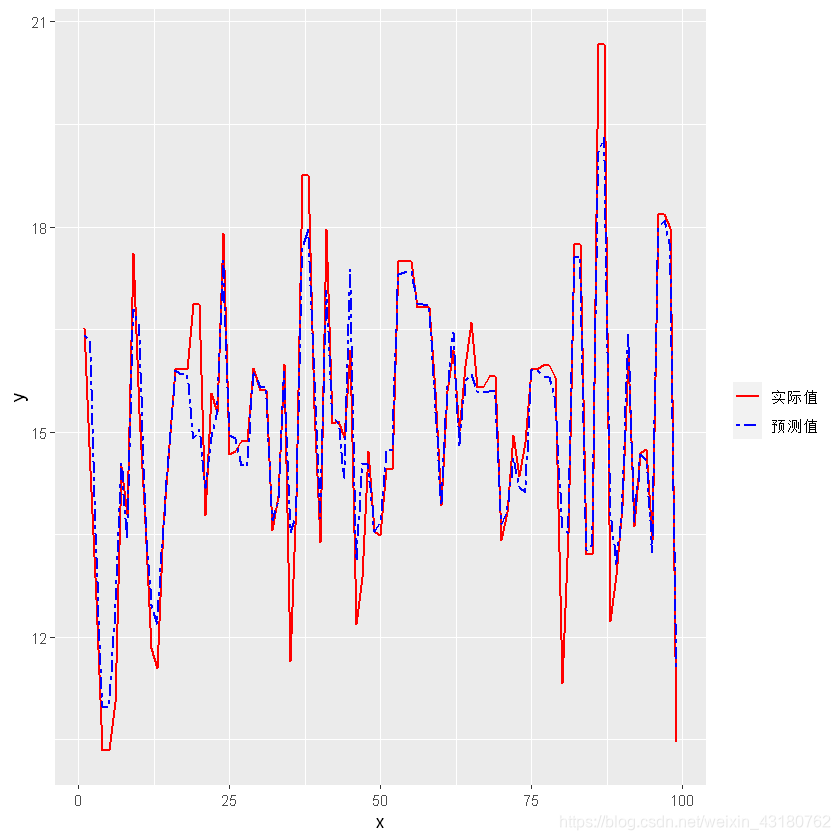
data5<-data.frame(total_pre,scoredata$晨星风险系数)
colnames(data5)<-c('预测','实际')
head(data5)

A data.frame: 6 × 2

	预测	实际
	<dbl>	<dbl>
1	15.32207	16.51
2	14.23500	14.44
3	12.85453	12.56
4	11.27575	10.35
5	11.26058	10.35
6	13.33599	11.05

df<-data.frame(x=c(1:99),y=data5$实际)
pre_y=data5$预测
head(df)
#训练集可视化
plot1 <- ggplot(data = df, aes(x = x)) + geom_line(aes(y = y, linetype = "实际值", colour = "实际值"), size = 0.8) ### 画实际值得曲线
plot2 <- plot1 + geom_line(aes(y = pre_y, linetype = "预测值", colour = "预测值"), size = 0.8) ### 画预测值曲线

plot2 + scale_linetype_manual(name = "", values = c("实际值" = "solid", "预测值" = "twodash")) +
  scale_colour_manual(name = "", values = c("实际值" = "red", "预测值" = "blue"))  ### 设置图例

A data.frame: 6 × 2

	x	y
	<int>	<dbl>
1	1	16.51
2	2	14.44
3	3	12.56
4	4	10.35
5	5	10.35
6	6	11.05

5.3 建立随机森林模型

library(readr)
library(VIM)
library(rpart)
library(rpart.plot)
library(Metrics)
library(ROCR)
library(tidyr)
library(randomForest)
library(ggRandomForests)
set.seed(123)
index <- sample(nrow(scoredata),round(0.7*nrow(scoredata)))
train_data <-scoredata[index,]
test_data <-scoredata[-index,]

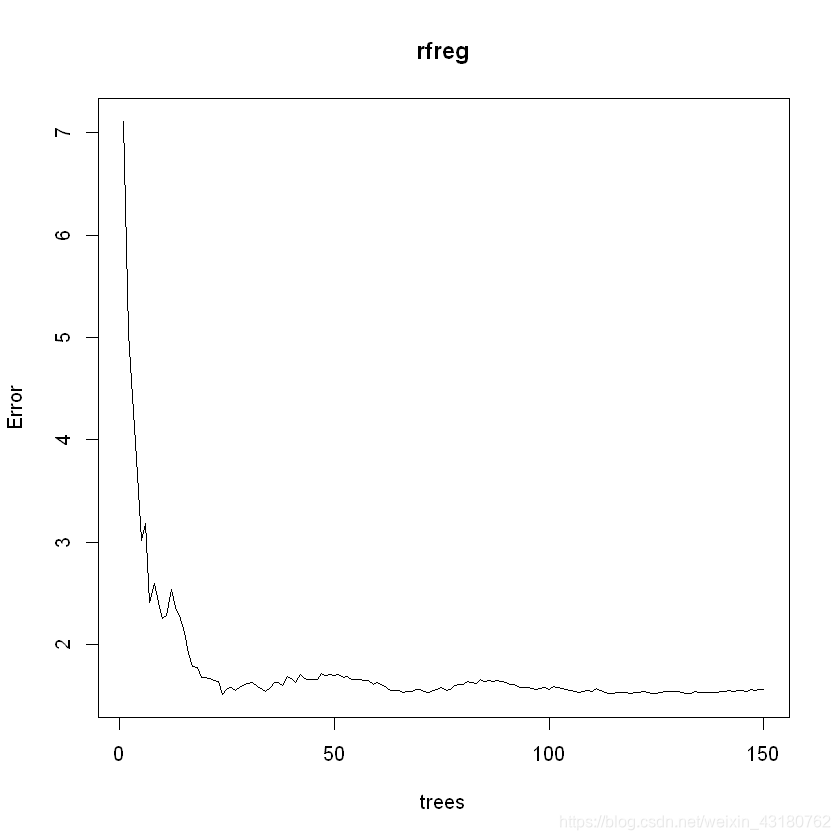
rfreg <- randomForest(晨星风险系数~.,data = train_data,ntree=150)
summary(rfreg)

                Length Class  Mode     
call              4    -none- call     
type              1    -none- character
predicted        69    -none- numeric  
mse             150    -none- numeric  
rsq             150    -none- numeric  
oob.times        69    -none- numeric  
importance       21    -none- numeric  
importanceSD      0    -none- NULL     
localImportance   0    -none- NULL     
proximity         0    -none- NULL     
ntree             1    -none- numeric  
mtry              1    -none- numeric  
forest           11    -none- list     
coefs             0    -none- NULL     
y                69    -none- numeric  
test              0    -none- NULL     
inbag             0    -none- NULL     
terms             3    terms  call     

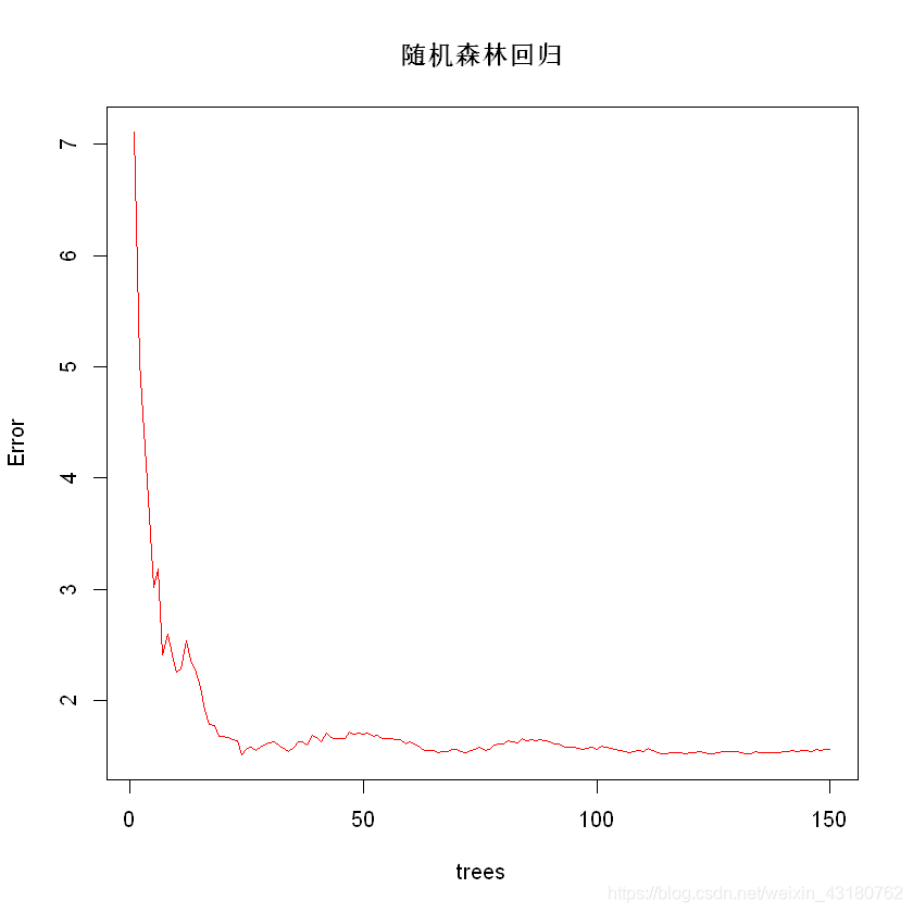
## 可视化模型随着树的增加误差OOB的变化
par(family = "STKaiti")
plot(rfreg,type = "l",col = "red",main = "随机森林回归")

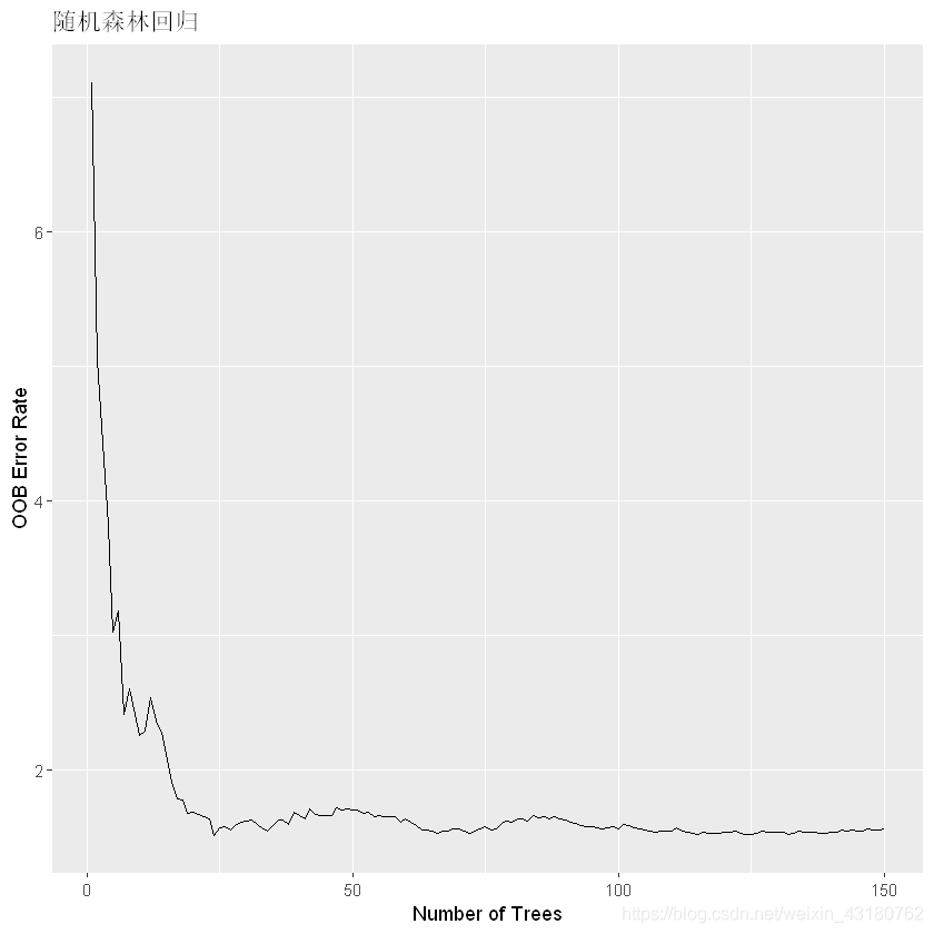
## 使用ggrandomforest包可视化误差
plot(gg_error(rfreg))+labs(title = "随机森林回归")

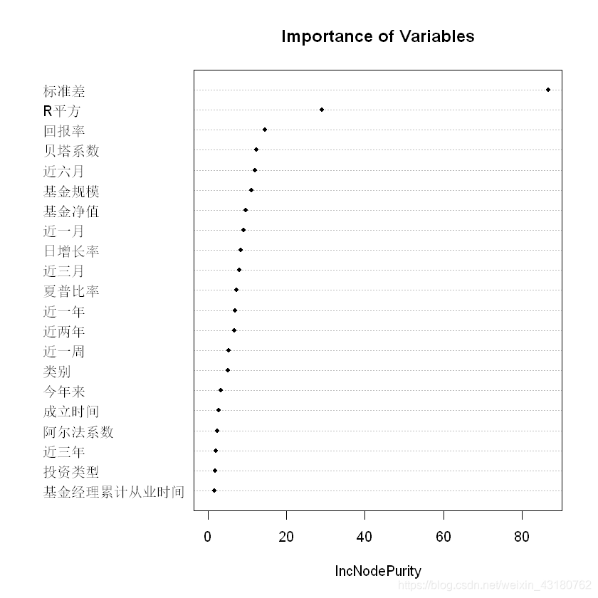
## 可视化变量的重要性
importance(rfreg)

A matrix: 21 × 1 of type dbl

	IncNodePurity
投资类型	1.873738
类别	5.235171
成立时间	2.823165
基金经理累计从业时间	1.664659
基金净值	9.702394
基金规模	11.184948
阿尔法系数	2.492178
贝塔系数	12.371313
R平方	29.013155
标准差	86.714834
夏普比率	7.370843
回报率	14.513756
日增长率	8.427672
近一周	5.300910
近一月	9.149165
近三月	8.074077
近六月	12.011001
今年来	3.402688
近一年	6.970955
近两年	6.801926
近三年	2.011527

varImpPlot(rfreg,pch = 20, main = "Importance of Variables")

## 对测试集进行预测，并计算 Mean Squared Error
rfpre <- predict(rfreg,test_data)
sprintf("均方根误差为: %f",mse(test_data$晨星风险系数,rfpre))

‘均方根误差为: 1.154161’

## 参数搜索,寻找合适的 mtry参数，训练更好的模型
## Tune randomForest for the optimal mtry parameter
set.seed(1234)
rftune <- tuneRF(x = test_data[,1:21],y = test_data$晨星风险系数,
                 stepFactor=1.5,ntreeTry = 150)

mtry = 7  OOB error = 2.296108 
Searching left ...
mtry = 5     OOB error = 2.187399 
0.04734515 0.05 
Searching right ...
mtry = 10     OOB error = 2.057613 
0.1038693 0.05 
mtry = 15     OOB error = 1.913855 
0.06986641 0.05 
mtry = 21     OOB error = 1.90867 
0.002709463 0.05 

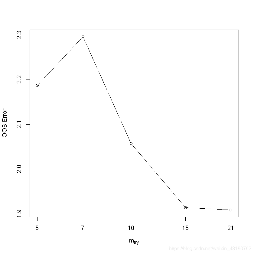
print(rftune)

   mtry OOBError
5     5 2.187399
7     7 2.296108
10   10 2.057613
15   15 1.913855
21   21 1.908670

## OOBError误差最小的mtry参数为6

## 建立优化后的随机森林回归模型
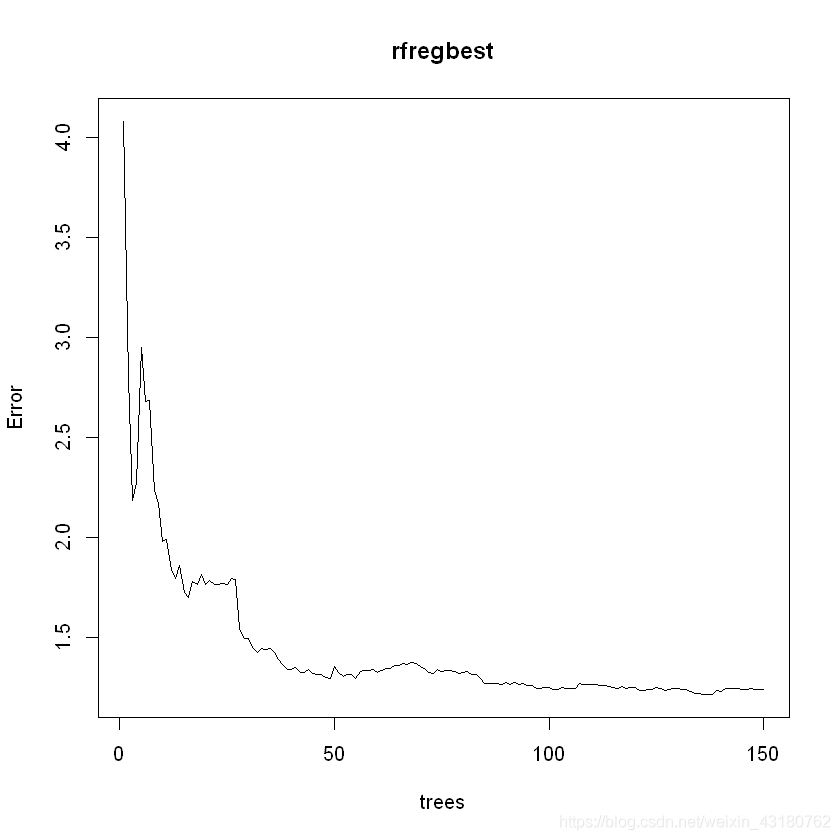
rfregbest <- randomForest(晨星风险系数~.,data = train_data,ntree=150,mtry = 15)

## 可视化两种模型随着树的增加误差OOB的变化
rfregerr <- as.data.frame(plot(rfreg))

colnames(rfregerr) <- "rfregerr"
rfregbesterr <- as.data.frame(plot(rfregbest))

#优化前后进行对比，可知优化后更好
colnames(rfregbesterr) <- "rfregbesterr"
plotrfdata <- cbind.data.frame(rfregerr,rfregbesterr)
plotrfdata$ntree <- 1:nrow(plotrfdata)
plotrfdata <- gather(plotrfdata,key = "Type",value = "Error",1:2)
ggplot(plotrfdata,aes(x = ntree,y = Error))+
  geom_line(aes(linetype = Type,colour = Type),size = 0.9)+
  theme(legend.position = "top")+
  ggtitle("随机森林回归模型")+
  theme(plot.title = element_text(hjust = 0.5))

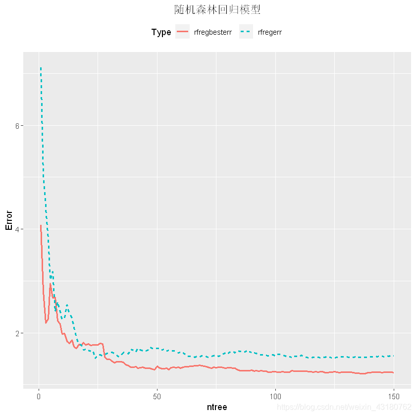
优化前后进行对比，可知优化后更好

## 使用优化后的随机森林回归模型，对测试集进行预测，并计算 Mean Squared Error
rfprebest <- predict(rfregbest,test_data[,1:21])
sprintf("优化后均方根误差为: %f",mse(test_data$晨星风险系数,rfprebest))

‘优化后均方根误差为: 1.046931’

## 使用优化后的随机森林回归模型，对测试集进行预测，并计算 Mean Squared Error
#全部数据
total <- predict(rfregbest,scoredata[,1:21])
sprintf("优化后均方根误差为: %f",mse(scoredata$晨星风险系数,total))

‘优化后均方根误差为: 0.460142’

#预测结果
totalpre<-data.frame(scoredata$晨星风险系数,total)
colnames(totalpre)<-c('实际','预测')
scoredata$预测<-total 
head(scoredata)

A tibble: 6 × 23

投资类型	类别	成立时间	基金经理累计从业时间	基金净值	基金规模	阿尔法系数	贝塔系数	R平方	标准差	...	近一周	近一月	近三月	近六月	今年来	近一年	近两年	近三年	晨星风险系数	预测
<chr>	<chr>	<dbl>	<dbl>	<dbl>	<dbl>	<dbl>	<dbl>	<dbl>	<dbl>	...	<dbl>	<dbl>	<dbl>	<dbl>	<dbl>	<dbl>	<dbl>	<dbl>	<dbl>	<dbl>
混合型	新能源	0.6666667	0.5	0.4277663	0.0148334010	0.6978110	0.20853081	0.5021714	0.6897133	...	0.93497537	0.86917462	0.6525212	1.0000000	0.8612148	0.9082674	0.7064660	0.6466077	16.51	16.41049
混合型	新能源	0.6666667	0.3	0.5308285	0.1119515885	1.0000000	0.21327014	0.5326766	0.6548623	...	0.57142857	0.49522740	0.5591613	0.6846304	0.6267391	1.0000000	1.0000000	1.0000000	14.44	16.32278
股票型	新能源	0.7333333	0.2	0.5970317	0.0508468322	0.8230112	0.12796209	0.5244148	0.4019112	...	0.68866995	0.68332398	0.4553170	0.6188619	0.5222260	0.7517509	0.6651190	0.7741506	12.56	13.20960
混合型	人工智能	0.7333333	0.2	0.2671426	0.0005165861	0.3852109	0.03791469	0.5776930	0.0786959	...	0.44137931	0.44637844	0.9430854	0.2003191	0.5714286	0.1747868	0.1620644	0.2584407	10.35	10.97816
混合型	国产软件	0.7333333	0.2	0.2671426	0.0005165861	0.3852109	0.03791469	0.5776930	0.0786959	...	0.44137931	0.44637844	0.9430854	0.2003191	0.5714286	0.1747868	0.1620644	0.2584407	10.35	10.97816
混合型	无人机	0.7333333	0.4	0.1183543	0.0113279953	0.4025627	0.12322275	0.4710306	0.4553120	...	0.06600985	0.07243122	0.2071892	0.2717603	0.1272480	0.3916717	0.2061483	0.2549260	11.05	12.38051

#预测结果
head(scoredata,25)

A tibble: 25 × 23

投资类型	类别	成立时间	基金经理累计从业时间	基金净值	基金规模	阿尔法系数	贝塔系数	R平方	标准差	...	近一周	近一月	近三月	近六月	今年来	近一年	近两年	近三年	晨星风险系数	预测
<chr>	<chr>	<dbl>	<dbl>	<dbl>	<dbl>	<dbl>	<dbl>	<dbl>	<dbl>	...	<dbl>	<dbl>	<dbl>	<dbl>	<dbl>	<dbl>	<dbl>	<dbl>	<dbl>	<dbl>
混合型	新能源	0.6666667	0.5	0.42776630	0.0148334010	0.6978110	0.20853081	0.5021714	0.6897133	...	0.93497537	0.86917462	0.6525212	1.0000000	0.8612148	0.9082674	0.7064660	0.6466077	16.51	16.41049
混合型	新能源	0.6666667	0.3	0.53082848	0.1119515885	1.0000000	0.21327014	0.5326766	0.6548623	...	0.57142857	0.49522740	0.5591613	0.6846304	0.6267391	1.0000000	1.0000000	1.0000000	14.44	16.32278
股票型	新能源	0.7333333	0.2	0.59703175	0.0508468322	0.8230112	0.12796209	0.5244148	0.4019112	...	0.68866995	0.68332398	0.4553170	0.6188619	0.5222260	0.7517509	0.6651190	0.7741506	12.56	13.20960
混合型	人工智能	0.7333333	0.2	0.26714259	0.0005165861	0.3852109	0.03791469	0.5776930	0.0786959	...	0.44137931	0.44637844	0.9430854	0.2003191	0.5714286	0.1747868	0.1620644	0.2584407	10.35	10.97816
混合型	国产软件	0.7333333	0.2	0.26714259	0.0005165861	0.3852109	0.03791469	0.5776930	0.0786959	...	0.44137931	0.44637844	0.9430854	0.2003191	0.5714286	0.1747868	0.1620644	0.2584407	10.35	10.97816
混合型	无人机	0.7333333	0.4	0.11835431	0.0113279953	0.4025627	0.12322275	0.4710306	0.4553120	...	0.06600985	0.07243122	0.2071892	0.2717603	0.1272480	0.3916717	0.2061483	0.2549260	11.05	12.38051
股票指数	无人机	0.7333333	0.3	0.19500282	0.0443895059	0.3473038	0.20379147	0.6111641	0.5306352	...	0.07783251	0.08197642	0.1562656	0.2283283	0.1214795	0.3263551	0.2011143	0.1823410	14.50	14.54577
股票型	新能源	0.7333333	0.0	0.26733045	0.1119515885	0.4813134	0.12796209	0.6121174	0.3035413	...	0.76157635	0.69118473	0.5401897	0.6505939	0.5917883	0.6903167	0.5095548	0.3933859	13.79	13.43880
股票型	国产软件	0.7333333	0.1	0.24760473	0.1657503413	0.3913508	0.08056872	0.8730007	0.6273187	...	0.66108374	0.65019652	0.6450325	0.4128701	0.6756023	0.3943362	0.4236352	0.2809138	17.61	16.79782
股票型	新能源	0.7333333	0.2	0.26714259	0.0113648943	0.7877736	0.24170616	0.5714437	0.6902754	...	0.99802956	1.00000000	0.4822766	0.8840631	0.5643027	0.6772229	0.6478178	0.7977420	15.28	16.51623
股票型	国产软件	0.8000000	0.5	0.20965621	0.0188184938	0.5192205	0.19431280	0.7505561	0.3569421	...	0.60985222	0.68388546	0.9760359	0.5263251	0.8683407	0.4491474	0.4209472	0.4477580	13.66	13.77112
股票型	新能源	0.8000000	0.4	0.13657712	0.0819526955	0.7471970	0.16587678	0.7132719	0.3209668	...	0.65221675	0.53733857	0.6694958	0.8860131	0.8758059	0.7599726	0.5252920	0.6761636	11.84	12.46147
股票型	新能源	0.8000000	0.9	0.10651888	0.0400723221	0.5315003	0.10426540	0.5916746	0.2647555	...	0.71428571	0.41774284	0.7124314	0.6800213	0.7037665	0.6877284	0.4395680	0.4162318	11.54	12.18295
股票型	新能源	0.8000000	1.0	0.17076836	0.0464558503	0.8035238	0.17061611	0.5589450	0.4952220	...	0.91330049	0.61650758	0.2456316	0.6865804	0.4285714	0.7797655	0.6864278	0.7502396	13.64	13.58897
股票型	国产软件	0.8000000	0.4	0.08932933	0.0162724623	0.5160171	0.01895735	0.8631501	0.3962901	...	0.54187192	0.49466592	0.4158762	0.2662648	0.4899898	0.2609622	0.3286741	0.3703270	14.81	14.81494
联接基金	智能穿戴	0.8000000	0.6	0.00000000	0.0121766724	0.2672184	0.06635071	0.9931151	0.4665542	...	0.43251232	0.47052218	0.7468797	0.2389647	0.4071938	0.2012789	0.1440301	0.1589094	15.91	15.89441
联接基金	人工智能	0.8000000	0.6	0.00000000	0.0121766724	0.2672184	0.06635071	0.9931151	0.4665542	...	0.43251232	0.47052218	0.7468797	0.2389647	0.6806922	0.2012789	0.1440301	0.1589094	15.91	15.84949
联接基金	生物识别	0.8000000	0.6	0.00000000	0.0121766724	0.2672184	0.06635071	0.9931151	0.4665542	...	0.43251232	0.47052218	0.7468797	0.2389647	0.6806922	0.2012789	0.1440301	0.1589094	15.91	15.84943
股票型	国产芯片	0.8000000	0.5	0.08190870	0.0205896461	0.4327282	0.03317536	0.8011863	0.4890388	...	0.43645320	0.54744526	0.4667998	0.2219465	0.5293519	0.2963611	0.2684620	0.3078070	16.87	14.90964
股票型	半导体	0.8000000	0.5	0.08190870	0.0205896461	0.4327282	0.03317536	0.8011863	0.4890388	...	0.43645320	0.54744526	0.4667998	0.2219465	0.5293519	0.2963611	0.2684620	0.3078070	16.87	15.03520
混合型	无人机	0.8000000	0.0	0.11516062	0.4116822257	0.4701014	0.23696682	0.6037496	0.6312535	...	0.00000000	0.23469961	0.3325012	0.2988832	0.1971496	0.5074604	0.3466595	0.3205347	13.78	14.17263
股票型	新能源	0.8000000	0.5	0.16607176	0.0436146268	0.7285104	0.22748815	0.6111641	0.5879708	...	0.68571429	0.62492981	0.5317024	0.6046800	0.7173397	0.8699756	0.7292410	0.7146128	15.57	14.91463
混合型	国产软件	0.8666667	0.8	0.29983092	0.1552341242	0.6444207	0.07109005	0.8896303	0.5705453	...	0.65320197	0.68613139	0.4418372	0.2714058	0.5320665	0.2520554	0.4030106	0.5286505	15.29	15.32525
联接基金	国产芯片	0.8000000	0.5	0.14181852	0.0127670566	0.4530166	0.11848341	0.9766974	0.6891512	...	0.52709360	0.59124088	0.7024463	0.3208651	0.6878181	0.3214829	0.3318020	0.3768239	17.91	17.50908
联接基金	人工智能	0.8000000	0.3	0.03304528	0.0140585218	0.2955152	0.04265403	0.9132507	0.4345138	...	0.34088670	0.42728804	0.7833250	0.1707144	0.6294537	0.1243149	0.1023899	0.1413356	14.67	14.95419

df<-data.frame(x=c(1:99),y=totalpre$实际)
pre_y=totalpre$预测
head(df)
#训练集可视化
plot1 <- ggplot(data = df, aes(x = x)) + geom_line(aes(y = y, linetype = "实际值", colour = "实际值"), size = 0.8) ### 画实际值得曲线
plot2 <- plot1 + geom_line(aes(y = pre_y, linetype = "预测值", colour = "预测值"), size = 0.8) ### 画预测值曲线

plot2 + scale_linetype_manual(name = "", values = c("实际值" = "solid", "预测值" = "twodash")) +
  scale_colour_manual(name = "", values = c("实际值" = "red", "预测值" = "blue"))  ### 设置图例

A data.frame: 6 × 2

	x	y
	<int>	<dbl>
1	1	16.51
2	2	14.44
3	3	12.56
4	4	10.35
5	5	10.35
6	6	11.05

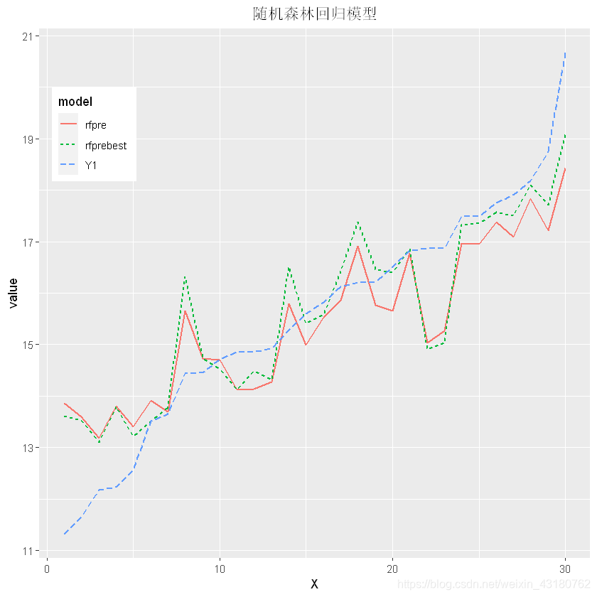
由于个别极端值，训练集中缺少这一部分较高的样本，故导致测试结果不尽人意，剔除这部分样本后，模型良好。

## 数据准备
index <- order(test_data$晨星风险系数)
X <- sort(index)
Y1 <- test_data$晨星风险系数[index]
rfpre2 <- rfpre[index]
rfprebest2 <- rfprebest[index]

plotdata <- data.frame(X = X,Y1 = Y1,rfpre =rfpre2,rfprebest = rfprebest2)
plotdata <- gather(plotdata,key="model",value="value",c(-X))

## 可视化模型的预测误差
ggplot(plotdata,aes(x = X,y = value))+
  geom_line(aes(linetype = model,colour = model),size = 0.8)+
  theme(legend.position = c(0.1,0.8),
        plot.title = element_text(hjust = 0.5))+
  ggtitle("随机森林回归模型")