6 单个神经元

6.5.1 交叉熵实验
假设有一个标签labels和一个网络输出值logits
（1）两次softmax实验
（2）两次交叉熵
（3）自建公式，将做两次softmax的值放到公式中得到正确的值

程序：

import tensorflow as tf

labels = [[0, 0, 1], [0, 1, 0]]
logits = [[2, 0.5, 6],
          [0.1, 0, 3]]
logits_scaled = tf.nn.softmax(logits)#计算softmax
logits_scaled2 = tf.nn.softmax(logits_scaled)

result1 = tf.nn.softmax_cross_entropy_with_logits(labels=labels, logits=logits)#计算交叉熵
result2 = tf.nn.softmax_cross_entropy_with_logits(labels=labels, logits=logits_scaled)
result3 = -tf.reduce_sum(labels * tf.log(logits_scaled), 1)#自己组合的函数

with tf.Session() as sess:
    print("scaled=", sess.run(logits_scaled))
    print("scaled2=", sess.run(logits_scaled2))  # 经过第二次的softmax后，分布概率会有变化

    print("rel1=", sess.run(result1), "\n")  # 正确的方式
    print("rel2=", sess.run(result2), "\n")  # 如果将softmax变换完的值放进去会，就相当于算第二次softmax的loss，所以会出错
    print("rel3=", sess.run(result3))
    print("--------------------------------------------------------")

结果：

scaled= [[0.01791432 0.00399722 0.97808844]
 [0.04980332 0.04506391 0.90513283]]
scaled2= [[0.21747023 0.21446465 0.56806517]
 [0.2300214  0.22893383 0.5410447 ]]
rel1= [0.02215516 3.0996735 ] 

rel2= [0.56551915 1.4743223 ] 

rel3= [0.02215518 3.0996735 ]

---

6.5.2 one_hot实验
对非one_hot编码为标签的数据进行交叉熵计算，比较其与one_hot编码的交叉熵之间的区别

程序：

import tensorflow as tf

labels = [[0, 0, 1], [0, 1, 0]]
logits = [[2, 0.5, 6],
          [0.1, 0, 3]]
logits_scaled = tf.nn.softmax(logits)#计算softmax
logits_scaled2 = tf.nn.softmax(logits_scaled)

result1 = tf.nn.softmax_cross_entropy_with_logits(labels=labels, logits=logits)#计算交叉熵
result2 = tf.nn.softmax_cross_entropy_with_logits(labels=labels, logits=logits_scaled)
result3 = -tf.reduce_sum(labels * tf.log(logits_scaled), 1)#自己组合的函数

with tf.Session() as sess:
    print("scaled=", sess.run(logits_scaled))
    print("scaled2=", sess.run(logits_scaled2))  # 经过第二次的softmax后，分布概率会有变化

    print("rel1=", sess.run(result1), "\n")  # 正确的方式
    print("rel2=", sess.run(result2), "\n")  # 如果将softmax变换完的值放进去会，就相当于算第二次softmax的loss，所以会出错
    print("rel3=", sess.run(result3))
    print("--------------------------------------------------------")


# 标签总概率为1
labels1 = [[0.4, 0.1, 0.5], [0.3, 0.6, 0.1]]
result4 = tf.nn.softmax_cross_entropy_with_logits(labels=labels1, logits=logits)
with tf.Session() as sess:
    print("rel4=", sess.run(result4), "\n")

结果：

6.5.3sparse交叉熵的使用
使用sparse_softmax_cross_entropy_with_logits函数，对非one_hot编码为标签的数据进行交叉熵计算，比较其与one_hot编码的交叉熵之间的区别

程序：

import tensorflow as tf

labels = [[0, 0, 1], [0, 1, 0]]
logits = [[2, 0.5, 6],
          [0.1, 0, 3]]
logits_scaled = tf.nn.softmax(logits)#计算softmax
logits_scaled2 = tf.nn.softmax(logits_scaled)

result1 = tf.nn.softmax_cross_entropy_with_logits(labels=labels, logits=logits)#计算交叉熵
result2 = tf.nn.softmax_cross_entropy_with_logits(labels=labels, logits=logits_scaled)
result3 = -tf.reduce_sum(labels * tf.log(logits_scaled), 1)#自己组合的函数

with tf.Session() as sess:
    print("scaled=", sess.run(logits_scaled))
    print("scaled2=", sess.run(logits_scaled2))  # 经过第二次的softmax后，分布概率会有变化

    print("rel1=", sess.run(result1), "\n")  # 正确的方式
    print("rel2=", sess.run(result2), "\n")  # 如果将softmax变换完的值放进去会，就相当于算第二次softmax的loss，所以会出错
    print("rel3=", sess.run(result3))
    print("--------------------------------------------------------")


# 标签总概率为1
labels1 = [[0.4, 0.1, 0.5], [0.3, 0.6, 0.1]]
result4 = tf.nn.softmax_cross_entropy_with_logits(labels=labels1, logits=logits)
with tf.Session() as sess:
    print("rel4=", sess.run(result4), "\n")
    print("--------------------------------------------------------")

# sparse
labels3 = [2, 1]  # 其实是0 1 2 三个类。等价 第一行 001 第二行 010
result5 = tf.nn.sparse_softmax_cross_entropy_with_logits(labels=labels3, logits=logits)
with tf.Session() as sess:
    print("rel5=", sess.run(result5), "\n")
    print("--------------------------------------------------------")

结果：

6.5.4 计算loss值

对前面的result1与softmax后的结果logits_scaled计算loss

程序：

import tensorflow as tf

labels = [[0, 0, 1], [0, 1, 0]]
logits = [[2, 0.5, 6],
          [0.1, 0, 3]]
logits_scaled = tf.nn.softmax(logits)#计算softmax
logits_scaled2 = tf.nn.softmax(logits_scaled)

result1 = tf.nn.softmax_cross_entropy_with_logits(labels=labels, logits=logits)#计算交叉熵
result2 = tf.nn.softmax_cross_entropy_with_logits(labels=labels, logits=logits_scaled)
result3 = -tf.reduce_sum(labels * tf.log(logits_scaled), 1)#自己组合的函数

with tf.Session() as sess:
    print("scaled=", sess.run(logits_scaled))
    print("scaled2=", sess.run(logits_scaled2))  # 经过第二次的softmax后，分布概率会有变化

    print("rel1=", sess.run(result1), "\n")  # 正确的方式
    print("rel2=", sess.run(result2), "\n")  # 如果将softmax变换完的值放进去会，就相当于算第二次softmax的loss，所以会出错
    print("rel3=", sess.run(result3))
    print("--------------------------------------------------------")


# 标签总概率为1
labels1 = [[0.4, 0.1, 0.5], [0.3, 0.6, 0.1]]
result4 = tf.nn.softmax_cross_entropy_with_logits(labels=labels1, logits=logits)
with tf.Session() as sess:
    print("rel4=", sess.run(result4), "\n")
    print("--------------------------------------------------------")

# sparse
labels3 = [2, 1]  # 其实是0 1 2 三个类。等价 第一行 001 第二行 010
result5 = tf.nn.sparse_softmax_cross_entropy_with_logits(labels=labels3, logits=logits)
with tf.Session() as sess:
    print("rel5=", sess.run(result5), "\n")
    print("--------------------------------------------------------")

# 注意！！！这个函数的返回值并不是一个数，而是一个向量，
# 如果要求交叉熵loss，我们要对向量求均值，
# 就是对向量再做一步tf.reduce_mean操作
loss = tf.reduce_mean(result1)
with tf.Session() as sess:
    print("loss=", sess.run(loss))
    print("--------------------------------------------------------")

labels4 = [[0, 0, 1], [0, 1, 0]]
loss2 = tf.reduce_mean(-tf.reduce_sum(labels4 * tf.log(logits_scaled), 1))
with tf.Session() as sess:
    print("loss2=", sess.run(loss2))

结果：

练习：
将上一章的代码改成使用sparse_softmax_cross_entropy_with_logits函数来计算交叉熵

程序：

from tensorflow.examples.tutorials.mnist import input_data
mnist = input_data.read_data_sets("F:/shendu/MNIST_data/")

print ('输入数据:',mnist.train.images)
print ('输入数据打shape:',mnist.train.images.shape)

import pylab 
im = mnist.train.images[1]
im = im.reshape(-1,28)
pylab.imshow(im)
pylab.show()


print ('输入数据打shape:',mnist.test.images.shape)
print ('输入数据打shape:',mnist.validation.images.shape)


import tensorflow as tf #导入tensorflow库

tf.reset_default_graph()
# tf Graph Input
x = tf.placeholder(tf.float32, [None, 784]) # mnist data维度 28*28=784
y = tf.placeholder(tf.int32, [None]) # 0-9 数字=> 10 classes

# Set model weights
W = tf.Variable(tf.random_normal([784, 10]))
b = tf.Variable(tf.zeros([10]))

z= tf.matmul(x, W) + b
# 构建模型
pred = tf.nn.softmax(z) # Softmax分类

# Minimize error using cross entropy
#cost = tf.reduce_mean(-tf.reduce_sum(y*tf.log(pred), reduction_indices=1))
cost = tf.reduce_mean(tf.nn.sparse_softmax_cross_entropy_with_logits(labels=y, logits=z))
#参数设置
learning_rate = 0.01
# 使用梯度下降优化器
optimizer = tf.train.GradientDescentOptimizer(learning_rate).minimize(cost)

training_epochs = 25
batch_size = 100
display_step = 1


# 启动session
with tf.Session() as sess:
    sess.run(tf.global_variables_initializer())# Initializing OP

    # 启动循环开始训练
    for epoch in range(training_epochs):
        avg_cost = 0.
        total_batch = int(mnist.train.num_examples/batch_size)
        # 遍历全部数据集
        for i in range(total_batch):
            batch_xs, batch_ys = mnist.train.next_batch(batch_size)
            # Run optimization op (backprop) and cost op (to get loss value)
            _, c = sess.run([optimizer, cost], feed_dict={x: batch_xs,
                                                          y: batch_ys})
            # Compute average loss
            avg_cost += c / total_batch
        # 显示训练中的详细信息
        if (epoch+1) % display_step == 0:
            print ("Epoch:", '%04d' % (epoch+1), "cost=", "{:.9f}".format(avg_cost))

    print( " Finished!")

结果：

Extracting F:/shendu/MNIST_data/train-images-idx3-ubyte.gz
Extracting F:/shendu/MNIST_data/train-labels-idx1-ubyte.gz
Extracting F:/shendu/MNIST_data/t10k-images-idx3-ubyte.gz
Extracting F:/shendu/MNIST_data/t10k-labels-idx1-ubyte.gz

输入数据: [[0. 0. 0. ... 0. 0. 0.]
 [0. 0. 0. ... 0. 0. 0.]
 [0. 0. 0. ... 0. 0. 0.]
 ...
 [0. 0. 0. ... 0. 0. 0.]
 [0. 0. 0. ... 0. 0. 0.]
 [0. 0. 0. ... 0. 0. 0.]]
输入数据打shape: (55000, 784)
输入数据打shape: (10000, 784)
输入数据打shape: (5000, 784)

Epoch: 0001 cost= 7.749131673
Epoch: 0002 cost= 3.810449805
Epoch: 0003 cost= 2.700252828
Epoch: 0004 cost= 2.193572711
Epoch: 0005 cost= 1.902135087
Epoch: 0006 cost= 1.709153523
Epoch: 0007 cost= 1.569791512
Epoch: 0008 cost= 1.463006385
Epoch: 0009 cost= 1.378214203
Epoch: 0010 cost= 1.308498062
Epoch: 0011 cost= 1.250179417
Epoch: 0012 cost= 1.200301619
Epoch: 0013 cost= 1.156732090
Epoch: 0014 cost= 1.118502057
Epoch: 0015 cost= 1.084579921
Epoch: 0016 cost= 1.053997789
Epoch: 0017 cost= 1.026608925
Epoch: 0018 cost= 1.001472130
Epoch: 0019 cost= 0.978647185
Epoch: 0020 cost= 0.957666033
Epoch: 0021 cost= 0.938214827
Epoch: 0022 cost= 0.920207297
Epoch: 0023 cost= 0.903384990
Epoch: 0024 cost= 0.887801428
Epoch: 0025 cost= 0.873080652
 Finished!

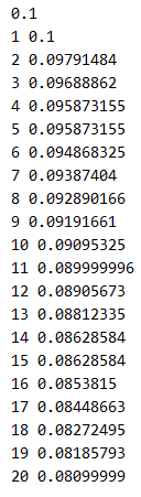
6.6.4 退化学习率的用法举例

定义一个学习率变量，将其衰减系数设置好，并设置好迭代循环的次数，将每次迭代运算的次数与学习率打印出来，观察学习率按照次数退化的现象

程序：

import tensorflow as tf

global_step = tf.Variable(0, trainable=False)

initial_learning_rate = 0.1 #初始学习率

#当前迭代到global_step步，学习率每一步都按照每10步缩小到0.9%的速度衰退
learning_rate = tf.train.exponential_decay(initial_learning_rate,
                                           global_step,
                                           decay_steps=10,decay_rate=0.9)
opt = tf.train.GradientDescentOptimizer(learning_rate)

add_global = global_step.assign_add(1)#定义一个op，令global_step加1完成计步
with tf.Session() as sess:
    tf.global_variables_initializer().run()
    print(sess.run(learning_rate))
    for i in range(20):#循环20步，将每步的学习率打印出来
        g, rate = sess.run([add_global, learning_rate])
        print(g,rate)

结果：

6.8.2 用Maxout网络实现MNIST分类
通过reduce_max函数对多个神经元的输出来计算Max值，将Max值当作输入按照神经元正反传播方向进行计算

程序：

from tensorflow.examples.tutorials.mnist import input_data
mnist = input_data.read_data_sets("F:/shendu/MNIST_data/")

print ('输入数据:',mnist.train.images)
print ('输入数据打shape:',mnist.train.images.shape)

import pylab
im = mnist.train.images[1]
im = im.reshape(-1,28)
pylab.imshow(im)
pylab.show()

print ('输入数据打shape:',mnist.test.images.shape)
print ('输入数据打shape:',mnist.validation.images.shape)
print ('----------------------------------------------')

import tensorflow as tf #导入tensorflow库

def max_out(inputs, num_units, axis=None):
    shape = inputs.get_shape().as_list()
    if shape[0] is None:
        shape[0] = -1
    if axis is None:  # Assume that channel is the last dimension
        axis = -1
    num_channels = shape[axis]
    if num_channels % num_units:
        raise ValueError('number of features({}) is not '
                         'a multiple of num_units({})'.format(num_channels, num_units))
    shape[axis] = num_units
    shape += [num_channels // num_units]
    outputs = tf.reduce_max(tf.reshape(inputs, shape), -1, keep_dims=False)
    return outputs

tf.reset_default_graph()
# tf Graph Input
x = tf.placeholder(tf.float32, [None, 784]) # mnist data维度 28*28=784
y = tf.placeholder(tf.int32, [None]) # 0-9 数字=> 10 classes

# Set model weights
W = tf.Variable(tf.random_normal([784, 100]))
b = tf.Variable(tf.zeros([100]))

z= tf.matmul(x, W) + b
#maxout = tf.reduce_max(z,axis= 1,keep_dims=True)

maxout= max_out(z, 50)

#在网络模型部分，添加一层Maxout,然后将Maxout作为maxsoft的交叉熵输入，学习率设为0.04，迭代次数设为200
#设置学习参数 Set model weights
W2 = tf.Variable(tf.truncated_normal([50, 10], stddev=0.1))
b2 = tf.Variable(tf.zeros([10]))
# 构建模型
#pred = tf.nn.softmax(tf.matmul(maxout, W2) + b2)
pred = tf.matmul(maxout, W2) + b2
# 构建模型
#pred = tf.nn.softmax(z) # Softmax分类

# Minimize error using cross entropy
#cost = tf.reduce_mean(-tf.reduce_sum(y*tf.log(pred), reduction_indices=1))
cost = tf.reduce_mean(tf.nn.sparse_softmax_cross_entropy_with_logits(labels=y, logits=pred))

#参数设置
learning_rate = 0.04
# 使用梯度下降优化器
optimizer = tf.train.GradientDescentOptimizer(learning_rate).minimize(cost)

training_epochs = 200
batch_size = 100
display_step = 1

# 启动session
with tf.Session() as sess:
    sess.run(tf.global_variables_initializer())# Initializing OP

    # 启动循环开始训练
    for epoch in range(training_epochs):
        avg_cost = 0.
        total_batch = int(mnist.train.num_examples/batch_size)
        # 遍历全部数据集
        for i in range(total_batch):
            batch_xs, batch_ys = mnist.train.next_batch(batch_size)
            # Run optimization op (backprop) and cost op (to get loss value)
            _, c = sess.run([optimizer, cost], feed_dict={x: batch_xs,
                                                          y: batch_ys})
            # Compute average loss
            avg_cost += c / total_batch
        # 显示训练中的详细信息
        if (epoch+1) % display_step == 0:
            print ("Epoch:", '%04d' % (epoch+1), "cost=", "{:.9f}".format(avg_cost))

    print( " Finished!")

结果：

Extracting F:/shendu/MNIST_data/train-images-idx3-ubyte.gz
Extracting F:/shendu/MNIST_data/train-labels-idx1-ubyte.gz
Extracting F:/shendu/MNIST_data/t10k-images-idx3-ubyte.gz
Extracting F:/shendu/MNIST_data/t10k-labels-idx1-ubyte.gz

输入数据: [[0. 0. 0. ... 0. 0. 0.]
 [0. 0. 0. ... 0. 0. 0.]
 [0. 0. 0. ... 0. 0. 0.]
 ...
 [0. 0. 0. ... 0. 0. 0.]
 [0. 0. 0. ... 0. 0. 0.]
 [0. 0. 0. ... 0. 0. 0.]]
输入数据打shape: (55000, 784)
输入数据打shape: (10000, 784)
输入数据打shape: (5000, 784)
----------------------------------------------

Epoch: 0001 cost= 1.831094528
Epoch: 0002 cost= 0.837515024
Epoch: 0003 cost= 0.671718355
Epoch: 0004 cost= 0.602337493
Epoch: 0005 cost= 0.550563356
Epoch: 0006 cost= 0.523226238
Epoch: 0007 cost= 0.499121306
Epoch: 0008 cost= 0.483308287
Epoch: 0009 cost= 0.462959923
Epoch: 0010 cost= 0.453428946
Epoch: 0011 cost= 0.441895107
Epoch: 0012 cost= 0.430031171
Epoch: 0013 cost= 0.420961845
Epoch: 0014 cost= 0.413285130
Epoch: 0015 cost= 0.408598027
Epoch: 0016 cost= 0.398942844
Epoch: 0017 cost= 0.393624266
Epoch: 0018 cost= 0.384940956
Epoch: 0019 cost= 0.381614986
Epoch: 0020 cost= 0.373610425
Epoch: 0021 cost= 0.370066817
Epoch: 0022 cost= 0.364395143
Epoch: 0023 cost= 0.361189684
Epoch: 0024 cost= 0.355336288
Epoch: 0025 cost= 0.349726792
Epoch: 0026 cost= 0.347820358
Epoch: 0027 cost= 0.344955071
Epoch: 0028 cost= 0.339195074
Epoch: 0029 cost= 0.335829557
Epoch: 0030 cost= 0.333333982
Epoch: 0031 cost= 0.329175626
Epoch: 0032 cost= 0.325885803
Epoch: 0033 cost= 0.322290837
Epoch: 0034 cost= 0.319717503
Epoch: 0035 cost= 0.316707550
Epoch: 0036 cost= 0.313841824
Epoch: 0037 cost= 0.311449403
Epoch: 0038 cost= 0.308557546
Epoch: 0039 cost= 0.305968530
Epoch: 0040 cost= 0.304210746
Epoch: 0041 cost= 0.299785262
Epoch: 0042 cost= 0.298015953
Epoch: 0043 cost= 0.296548855
Epoch: 0044 cost= 0.293712433
Epoch: 0045 cost= 0.291924013
Epoch: 0046 cost= 0.288433217
Epoch: 0047 cost= 0.287236811
Epoch: 0048 cost= 0.286207905
Epoch: 0049 cost= 0.283707174
Epoch: 0050 cost= 0.281909256
Epoch: 0051 cost= 0.279137198
Epoch: 0052 cost= 0.277186460
Epoch: 0053 cost= 0.275229350
Epoch: 0054 cost= 0.273223751
Epoch: 0055 cost= 0.272368153
Epoch: 0056 cost= 0.270435052
Epoch: 0057 cost= 0.268903814
Epoch: 0058 cost= 0.266802683
Epoch: 0059 cost= 0.265594411
Epoch: 0060 cost= 0.264045720
Epoch: 0061 cost= 0.261642672
Epoch: 0062 cost= 0.260362809
Epoch: 0063 cost= 0.259614022
Epoch: 0064 cost= 0.256968227
Epoch: 0065 cost= 0.256806671
Epoch: 0066 cost= 0.253737082
Epoch: 0067 cost= 0.251577917
Epoch: 0068 cost= 0.251639100
Epoch: 0069 cost= 0.249998931
Epoch: 0070 cost= 0.248551697
Epoch: 0071 cost= 0.247193317
Epoch: 0072 cost= 0.247242698
Epoch: 0073 cost= 0.242939282
Epoch: 0074 cost= 0.244006023
Epoch: 0075 cost= 0.241111588
Epoch: 0076 cost= 0.239570004
Epoch: 0077 cost= 0.239140056
Epoch: 0078 cost= 0.238168426
Epoch: 0079 cost= 0.237239161
Epoch: 0080 cost= 0.234841672
Epoch: 0081 cost= 0.234336329
Epoch: 0082 cost= 0.233081204
Epoch: 0083 cost= 0.232232782
Epoch: 0084 cost= 0.230691200
Epoch: 0085 cost= 0.229409278
Epoch: 0086 cost= 0.230101153
Epoch: 0087 cost= 0.228259589
Epoch: 0088 cost= 0.225365908
Epoch: 0089 cost= 0.224674840
Epoch: 0090 cost= 0.224802138
Epoch: 0091 cost= 0.222409938
Epoch: 0092 cost= 0.222278961
Epoch: 0093 cost= 0.220977059
Epoch: 0094 cost= 0.220964662
Epoch: 0095 cost= 0.219540731
Epoch: 0096 cost= 0.218384535
Epoch: 0097 cost= 0.217279785
Epoch: 0098 cost= 0.216344066
Epoch: 0099 cost= 0.215243163
Epoch: 0100 cost= 0.214545646
Epoch: 0101 cost= 0.213273921
Epoch: 0102 cost= 0.212897576
Epoch: 0103 cost= 0.211499919
Epoch: 0104 cost= 0.210271833
Epoch: 0105 cost= 0.209163501
Epoch: 0106 cost= 0.209519286
Epoch: 0107 cost= 0.207314329
Epoch: 0108 cost= 0.207046347
Epoch: 0109 cost= 0.205767930
Epoch: 0110 cost= 0.205214316
Epoch: 0111 cost= 0.204563683
Epoch: 0112 cost= 0.204319949
Epoch: 0113 cost= 0.202254281
Epoch: 0114 cost= 0.201350747
Epoch: 0115 cost= 0.200614012
Epoch: 0116 cost= 0.199791828
Epoch: 0117 cost= 0.199906992
Epoch: 0118 cost= 0.199054424
Epoch: 0119 cost= 0.198625167
Epoch: 0120 cost= 0.196974152
Epoch: 0121 cost= 0.195345124
Epoch: 0122 cost= 0.195541776
Epoch: 0123 cost= 0.195379050
Epoch: 0124 cost= 0.193745826
Epoch: 0125 cost= 0.193098677
Epoch: 0126 cost= 0.191266442
Epoch: 0127 cost= 0.191914391
Epoch: 0128 cost= 0.191295051
Epoch: 0129 cost= 0.189877646
Epoch: 0130 cost= 0.190133466
Epoch: 0131 cost= 0.188530851
Epoch: 0132 cost= 0.188043243
Epoch: 0133 cost= 0.187539196
Epoch: 0134 cost= 0.186910501
Epoch: 0135 cost= 0.186791751
Epoch: 0136 cost= 0.185061639
Epoch: 0137 cost= 0.184676404
Epoch: 0138 cost= 0.185102803
Epoch: 0139 cost= 0.183270461
Epoch: 0140 cost= 0.183129580
Epoch: 0141 cost= 0.182038182
Epoch: 0142 cost= 0.181006520
Epoch: 0143 cost= 0.180876898
Epoch: 0144 cost= 0.180306361
Epoch: 0145 cost= 0.179016846
Epoch: 0146 cost= 0.179368026
Epoch: 0147 cost= 0.177696267
Epoch: 0148 cost= 0.178141219
Epoch: 0149 cost= 0.176431095
Epoch: 0150 cost= 0.176945710
Epoch: 0151 cost= 0.175768193
Epoch: 0152 cost= 0.175612516
Epoch: 0153 cost= 0.173862670
Epoch: 0154 cost= 0.174989760
Epoch: 0155 cost= 0.173892279
Epoch: 0156 cost= 0.172517994
Epoch: 0157 cost= 0.172950397
Epoch: 0158 cost= 0.171439644
Epoch: 0159 cost= 0.171710244
Epoch: 0160 cost= 0.170230712
Epoch: 0161 cost= 0.168839366
Epoch: 0162 cost= 0.169254420
Epoch: 0163 cost= 0.168633991
Epoch: 0164 cost= 0.168330751
Epoch: 0165 cost= 0.167662011
Epoch: 0166 cost= 0.166983845
Epoch: 0167 cost= 0.166347573
Epoch: 0168 cost= 0.166072966
Epoch: 0169 cost= 0.164887908
Epoch: 0170 cost= 0.164859345
Epoch: 0171 cost= 0.164567883
Epoch: 0172 cost= 0.163842578
Epoch: 0173 cost= 0.163483603
Epoch: 0174 cost= 0.162623162
Epoch: 0175 cost= 0.163231879
Epoch: 0176 cost= 0.161974811
Epoch: 0177 cost= 0.162120592
Epoch: 0178 cost= 0.161084283
Epoch: 0179 cost= 0.160400136
Epoch: 0180 cost= 0.160386801
Epoch: 0181 cost= 0.158510944
Epoch: 0182 cost= 0.159255647
Epoch: 0183 cost= 0.158561282
Epoch: 0184 cost= 0.158412425
Epoch: 0185 cost= 0.157556693
Epoch: 0186 cost= 0.156945509
Epoch: 0187 cost= 0.157517383
Epoch: 0188 cost= 0.156452993
Epoch: 0189 cost= 0.155194256
Epoch: 0190 cost= 0.155830007
Epoch: 0191 cost= 0.155408271
Epoch: 0192 cost= 0.153861681
Epoch: 0193 cost= 0.153714444
Epoch: 0194 cost= 0.153413276
Epoch: 0195 cost= 0.152880426
Epoch: 0196 cost= 0.152503436
Epoch: 0197 cost= 0.152214802
Epoch: 0198 cost= 0.151338356
Epoch: 0199 cost= 0.150809068
Epoch: 0200 cost= 0.150530687
 Finished!