python气象处理第三弹-绘制气象站点分布

python气象处理第三弹-绘制气象站点分布

---

---

前言

在书写科研论文的研究区域的部分时，常常需要对研究区域的地形、气象观测站点等信息的进行图片形式的展现。因此参考Python可视化中国区域地面气象要素驱动数据集—以黄河流域为例绘制出了中国气象站点和黄河流域分布图。

---

一、下载并转换中国气象站点数据？

下载链接中国气象要素逐日站点观测数据集

查询发现下载的为shp信息

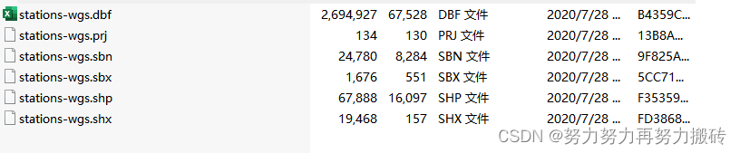
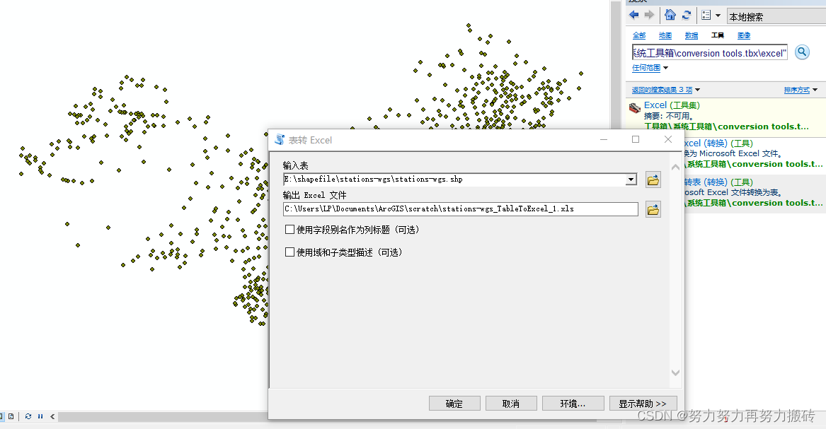
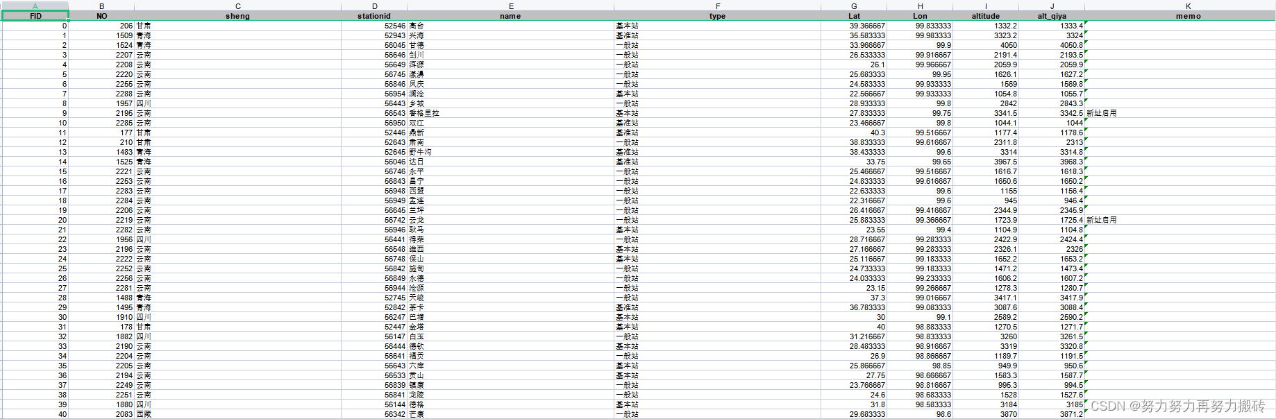
因此用arcmap打开文件查询站点信息如下

利用上图转换工具将.dbf转换成excel .xls数据方便利用python读取站点数据并绘图

二、使用步骤

1.引入库

代码如下（示例）：

import warnings
warnings.filterwarnings("ignore")
import matplotlib as mpl
import matplotlib.pyplot as plt
import cartopy.crs as ccrs
import cartopy.feature as cfeat
import cartopy.mpl.ticker as cticker
import matplotlib.ticker as mticker
from cartopy.mpl.gridliner import LONGITUDE_FORMATTER, LATITUDE_FORMATTER
import pandas as pd
import numpy as np
from matplotlib.path import Path
from matplotlib.patches import PathPatch
import shapefile
import xarray as xr
import netCDF4 as nc
from cartopy.mpl.gridliner import LONGITUDE_FORMATTER, LATITUDE_FORMATTER
from matplotlib.colors import BoundaryNorm, ListedColormap,LinearSegmentedColormap
from cartopy.io.shapereader import Reader
import pandas as pd

2.读入数据

代码如下（示例）：

#读取全球地形数据
import xarray as xr# 导入xarray库
ds = xr.open_dataset('E:/CORDEX-TP/DATA/ETOPO2v2c_f4.nc')# 读取全球地形数据
x=ds.x
y=ds.y
z=ds.z
leftlat=np.where(y == 14.75)
rightlat=np.where(y == 55.25)
leftlon=np.where(x == 64.75)
rightlon=np.where(x == 140.25)
#读取中国站点数据
data = pd.read_csv("china_station.csv")
data.head
#绘制站点分布图[站点分布](https://zhuanlan.zhihu.com/p/411537086)
from matplotlib import rcParams
import cmaps
config = {"font.family":'Times New Roman',"font.size":12,"mathtext.fontset":'stix'}
rcParams.update(config)
region=[70,140,15,55]
fig=plt.figure(dpi=600,figsize=(12,6))
proj=ccrs.PlateCarree()
ax = plt.axes(projection = proj)
ax.set_extent(region, crs = proj)
ax.set_xticks(np.arange(region[0], region[1] + 1, 5), crs = proj)
ax.set_yticks(np.arange(region[-2], region[-1] + 1, 2), crs = proj)
ax.xaxis.set_major_formatter(LongitudeFormatter(zero_direction_label=False))
ax.yaxis.set_major_formatter(LatitudeFormatter())
# Add 中国十段线shp
ax.add_geometries(Reader(r'E:/shapefile/china_shp/china10.shp').geometries(),ccrs.PlateCarree(),facecolor='none',edgecolor='k',linewidth=0.2)
c11=ax.contourf(lon,lat,dem,np.arange(0,8000,500),extend='both',transform=ccrs.PlateCarree(),cmap=cmaps.MPL_terrain)
#clip=shp2clip(c11,ax,'E:/shapefile/china_shp/china10')
cbar=plt.colorbar(c11,shrink=0.75,aspect=20,fraction=.03,pad=0.02)   #aspect控制bar宽度，fraction控制大小比例,pad控制与图的距离
cbar.set_ticks(np.arange(0,8000,500))            #设置colorbar范围和刻度标记间隔
cbar.ax.tick_params(labelsize=12, direction='in', right=False)
font3={'family':'SimHei','size':4,'color':'k'}
plt.scatter(data1['Lon'].values,data1['Lat'].values,marker='o',s=6,color ="k")
for i, j, k in list(zip(data1['Lon'].values, data1['Lat'].values, data1['name'].values)):
    plt.text(i-0.2,j-0.3,k,fontdict=font3)
ax.set_title('1979—2018年中国区域地面气象要素（气温）驱动数据集. 单位：K',{'family':'simhei','size':14,'color':'k'})
ax0 = plt.gca()   #获取边框
ax0.outline_patch.set_linewidth(0.5)    #修改边框粗细
#出图
plt.savefig('plot3.png',dpi=600)
plt.show()
#绘制青藏高原气象站点图
import frykit.plot as fplt
from matplotlib import rcParams
import cmaps
config = {"font.family":'Times New Roman',"font.size":12,"mathtext.fontset":'stix'}
rcParams.update(config)
region=[65, 114,20, 50]
fig=plt.figure(dpi=600,figsize=(12,6))
proj=ccrs.PlateCarree()
ax = plt.axes(projection = proj)
ax.set_extent(region, crs = proj)
ax.set_xticks(np.arange(region[0], region[1] + 1, 5), crs = proj)
ax.set_yticks(np.arange(region[-2], region[-1] + 1, 2), crs = proj)
ax.xaxis.set_major_formatter(LongitudeFormatter(zero_direction_label=False))
ax.yaxis.set_major_formatter(LatitudeFormatter())
# Add 中国十段线shp
shp_path = 'E:/shapefile/青藏高原/青藏高原边界数据总集/TPBoundary_new(2021)/'
shpfile=shp_path+'TPBoundary_new(2021).shp'
ax.add_feature(cfeat.RIVERS,  color = 'grey',zorder=1,edgecolor='black') 
ax.add_geometries(Reader(r'E:/shapefile/青藏高原/青藏高原边界数据总集/TPBoundary_new(2021)/TPBoundary_new(2021).shp').geometries(),ccrs.PlateCarree(),facecolor='none',edgecolor='k',linewidth=0.2)
ax.add_geometries(Reader(r'E:/shapefile/青藏高原/青藏高原省级行政边界（2015）/青藏高原省级行政边界.shp').geometries(),ccrs.PlateCarree(),facecolor='none',edgecolor='k',linewidth=0.2)
#ax.add_geometries(Reader(r'E:/shapefile/hhriver/jichu/黄河干流epsg4324.shp').geometries(),ccrs.PlateCarree(),facecolor='none',edgecolor='k',linewidth=0.5)
c11=ax.contourf(lon2,lat2,dem2,np.arange(0,8000,500),extend='both',transform=ccrs.PlateCarree(),cmap=cmaps.MPL_terrain)
# 添加指北针和比例尺.
fplt.add_north_arrow(ax, (0.1, 0.85))
fplt.add_map_scale(ax, (0.5, 0.1), length=1000, ticks=[0, 250,500, 1000])
font3={'family':'SimHei','size':4,'color':'k'}
plt.scatter(data['Lon.'].values,data['Lat.'].values,marker='o',s=6,color ="k")
position1=fig.add_axes([0.2, 0.01, 0.6, 0.018])#位置[左,下,右,上]  0.25, 0.35, 0.5, 0.014
cb=plt.colorbar(c11,cax=position1,orientation='horizontal')#方向
position1.set_title('Topography(m)',loc = 'center',fontsize=10,weight = 'normal')    
cb.set_ticks(np.arange(0,8000,500))            #设置colorbar范围和刻度标记间隔
position1.set_title('Topography(m)',loc = 'center',fontsize=10,weight = 'normal')
cbar.ax.tick_params(labelsize=12, direction='in', right=False)
#clip=shp2clip(c11,ax,shpfile)
'''for i, j, k in list(zip(data['Lon.'].values, data['Lat.'].values, data['Name'].values)):
    plt.text(i-0.2,j-0.3,k,fontdict=font3)
#ax.set_title('青藏高原站点分布.单位：m',{'family':'simhei','size':14,'color':'k'})
ax0 = plt.gca()   #获取边框
ax0.outline_patch.set_linewidth(0.5)    #修改边框粗细'''
#出图
plt.savefig('tpstation.png',dpi=600)
plt.show()

Cartopy 绘制填色地图-添加指北针

3.frykit说明

pip install frykit

其中引入了一个frykit包，这是参考了气象备忘录公众号关于cartopy系列文章的说明frykit说明

• 为兰伯特投影的 GeoAxes 添加刻度

import frykit.plot as fplot

crs = ccrs.LambertConformal(central_longitude=105, standard_parallels=(25, 47))
ax = fig.add_subplot(111, projection=crs)

fplt.set_extent_and_ticks(
    ax, extents=[74, 136, 14, 56],
    xticks=np.arange(50, 161, 10),
    yticks=np.arange(0, 71, 10),
    grid=True, lw=0.5, ls='--', color='gray'
)

• 获取代表中国行政区划的多边形对象

import frykit.shp as fshp

country = fshp.get_cnshp(level='国')
provinces = fshp.get_cnshp(level='省')

行政区划的 shapefile 文件来自 ChinaAdminDivisonSHP 项目，坐标已从 GCJ-02 坐标系处理到了 WGS84 坐标系上。

• 在 Axes 或 GeoAxes 上直接绘制中国省界和十段线

fplt.add_cn_province(ax, lw=0.3)
fplt.add_nine_line(ax, lw=0.5)

• 添加自备的多边形对象并填色

pc = fplt.add_polygons(
    ax, polygons, ccrs.PlateCarree(), array=data,
    cmap=cmap, norm=norm, ec='k', lw=0.4
)
cbar = fig.colorbar(pc, ax=ax)

• 用国界裁剪等值线填色图

cf = ax.contourf(
    lon, lat, data, levels, cmap='turbo',
    extend='both', transform=ccrs.PlateCarree()
)
fplt.clip_by_cn_border(cf, fix=True)

• 添加指北针和比例尺

fplt.add_north_arrow(ax, (0.95, 0.9))
fplt.add_map_scale(ax, (0.1, 0.1), length=1000, ticks=[0, 500, 1000])

• 定位南海地图

sub = fig.add_axes(ax.get_position(), projection=crs_map)
<plotting on sub>
fplt.locate_sub_axes(ax, sub, shrink=0.4)
 

总结

绘制站点分布主要分为三大步骤：

• 用contourf绘制地形填充
• 用scatter绘制站点信息
• 用maskout掩膜感兴趣的区域