从头理解线性回归学习笔记

从零认识线性回归

1.线性回归模型

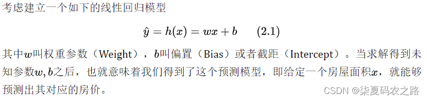
（1）了解线性回归模型

总体上呈现线性增长的趋势。如：房价预测

 

 

（2）sklearn简介

是一个开源的机器学习框架，例如线性回归、逻辑回归、决策树等等。

安装python包

pip install sklearn matplotlib

 线性回归示例代码

#导包
import numpy as np
from sklearn.linear_model import LinearRegression
import matplotlib.pyplot as plt

#制作样本  训练集
def make_data():
    np.random.seed(20)
    x = np.random.rand(100) * 30 + 50  # 面积
    noise = np.random.rand(100) * 50    #加入一定的噪音（误差）
    y = x * 8 - 127 - noise              # 价格
    return x,y


#定义模型并求解
def main(x, y):
    model = LinearRegression()            # 定义模型
    x = np.reshape(x, (-1, 1))  #把x变成[n,1]的形状，至于n到底是多少，将通过np.reshape函数自己推导得出
    model.fit(np.reshape(x, (-1, 1)), y)# 求解模型  用训练器数据拟合分类器模型
    y_pre = model.predict(x) # 预测
    print(y_pre)


#运行结果
if __name__ == '__main__':
    x, y = make_data()
    main(x, y)   

2.多变量线性回归

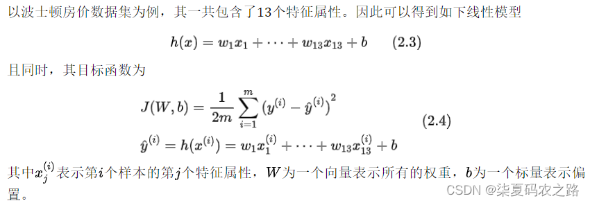
包含有多个特征的线性回归就叫做多变量线性回归。

 代码示例：

#导入数据集
def load_data():
    data = load_boston()
    x = data.data
    y = data.target
    return x, y


#求解与结果（训练模型与输出相应的权重参数和预测值）
def train(x, y):
    model = LinearRegression()
    model.fit(x,y)
    print("权重为：",model.coef_,"偏置为：",model.intercept_)
    print("第12个房屋的预测和真实价格：",model.predict(x[12,:].reshape(1,-1)))

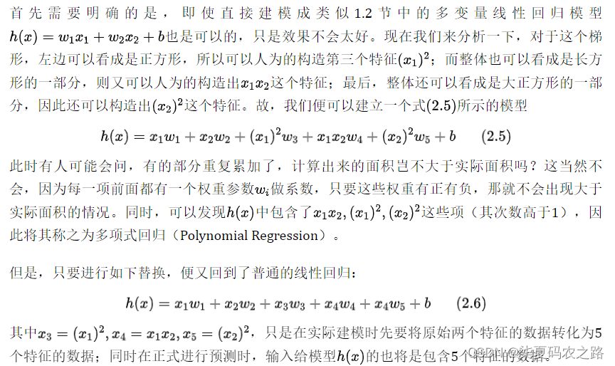
3.多项式回归

 示例代码：

#1特征转化
from sklearn.preprocessing import PolynomialFeatures
a = [[3, 4], [2, 3]]  
model = PolynomialFeatures(degree=2,include_bias=False) #degree表示变化维度2，include_bias是否添加一列全部等于1的偏置项
b = model.fit_transform(a) #对数据先进行拟合，然后标准化
print(b)


#2构造数据集
def make_data():
    np.random.seed(10) #生成指定随机数
    x1 = np.random.randint(5, 10, 50).reshape(50, 1)#根据参数中指定范围生成随机整数
    x2 = np.random.randint(10, 16, 50).reshape(50, 1)
    x,y = np.hstack((x1, x2)), 0.5 * (x1 + x2) * x1 #将参数元组的元素组按水平方向进行叠加
    return x, y

#根据上述代码便得到了一个50行2列的样本数据，其中第一列为上底，第二列为下底。np.hstack的作用是将两个50行1列的向量合并成一个50行2列的矩阵。

#3建模求解与结果
def train(x, y):
    poly = PolynomialFeatures(degree=2, include_bias=False)  #PolynomialFeatures构建特征
    x_mul = poly.fit_transform(x)
    model = LinearRegression()
    model.fit(x_mul, y)
    print("权重为：", model.coef_)#[[0.  0.  0.5   0.5   0]]
    print("偏置为：", model.intercept_) # [0.]

 4.回归模型评估

在回归任务（对连续值的预测）中，常见的评估指标（Metric）有平均绝对误差（Mean Absolute Error,MAE）、均方误差（Mean Square Error,MSE）、均方根误差（Root Mean Square Error,RMSE）、平均绝对百分比误差（Mean Absolute Percentage Error,MAPE）和决定系数（Coefficient of Determination），其中用得最为广泛的就是MAE和MSE。

（1）MAE平均绝对误差

 

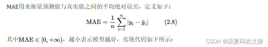
def MAE(y, y_pre):
    return np.mean(np.abs(y - y_pre))

（2）MSE均方误差

 

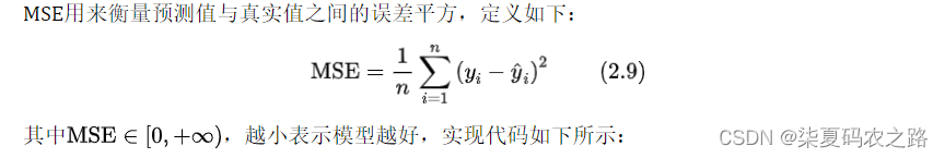
def MSE(y, y_pre):
    return np.mean((y - y_pre) ** 2)

（3）RMSE均方根误差

 

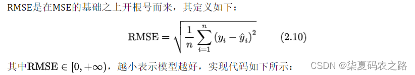
def RMSE(y, y_pre): 
    return np.sqrt(MSE(y, y_pre))

（4）MAPE平均绝对百分比误差

 

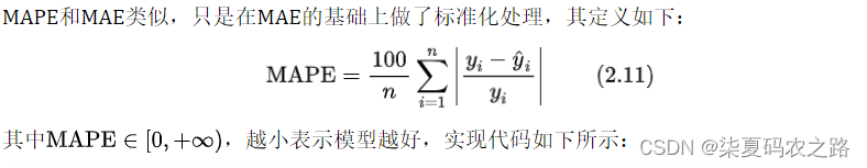
def MAPE(y, y_pre):
    return np.mean(np.abs((y - y_pre) / y))

 （5）

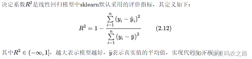
def R2(y, y_pre):
    u = np.sum((y - y_pre) ** 2)
    v = np.sum((y - np.mean(y_pre)) ** 2)
    return 1 - (u / v)

回归指标示例代码

def train(x, y):
    model = LinearRegression()
    model.fit(x, y)
    y_pre = model.predict(x) 

5.梯度下降

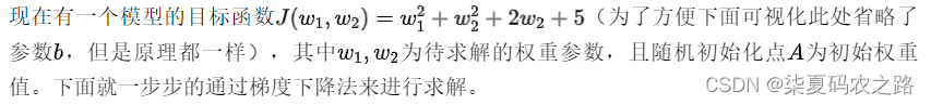
梯度下降算法的目的是最小化目标函数，也就是一个求解的工具。当目标函数取到（或接近）全局最小值时，我们也就求解得到了模型所对应的参数。

 梯度下降完成代码：

def cost_function(w1, w2):
    J = w1 ** 2 + w2 ** 2 + 2 * w2 + 5
    return J
def compute_gradient(w1, w2):
    return [2 * w1, 2 * w2 + 2]

def gradient_descent():
    w1, w2 = -2, 3
    jump_points = [[w1, w2]]
    costs = [cost_function(w1, w2)]
    step = 0.1
    print("P:({},{})".format(w1, w2), end=' ')
    for i in range(20):
        gradients = compute_gradient(w1, w2)
        w1 = w1 - step * gradients[0]
        w2 = w2 - step * gradients[1]
        jump_points.append([w1, w2])
        costs.append(cost_function(w1, w2))
        print("P{}:({},{})".format(i + 1, round(w1, 3), round(w2, 3)), end=' ')
    return jump_points, costs

if __name__ == '__main__':
    jump_points, costs = gradient_descent()
    plot_surface_and_jump_points(jump_points, costs)

 以上信息均为自己的学习笔记，来源于网络！！