


1 逻辑回归的介绍和应用
1.1 逻辑回归的介绍
逻辑回归(Logistic regression,简称LR)虽然其中带有"回归"两个字,但逻辑回归其实是一个分类模型,并且广泛应用于各个领域之中。虽然现在深度学习相对于这些传统方法更为火热,但实则这些传统方法由于其独特的优势依然广泛应用于各个领域中。
而对于逻辑回归而且,最为突出的两点就是其模型简单和模型的可解释性强。
逻辑回归模型的优劣势:
- 优点:实现简单,易于理解和实现;计算代价不高,速度很快,存储资源低;
- 缺点:容易欠拟合,分类精度可能不高
逻辑回归 原理简介:
Logistic回归虽然名字里带“回归”,但是它实际上是一种分类方法,主要用于两分类问题(即输出只有两种,分别代表两个类别),所以利用了Logistic函数(或称为Sigmoid函数),函数形式为:
l
o
g
i
(
z
)
=
1
1
+
e
−
z
logi(z)=\frac{1}{1+e^{-z}}
logi(z)=1+e−z1
其对应的函数图像可以表示如下:
import numpy as np
import matplotlib.pyplot as plt
x = np.arange(-5,5,0.01)
y = 1/(1+np.exp(-x))

plt.plot(x,y)
plt.xlabel('z')
plt.ylabel('y')
plt.grid()
plt.show()
 通过上图我们可以发现 Logistic 函数是单调递增函数,并且在z=0的时候取值为0.5,并且
l
o
g
i
(
⋅
)
logi(\cdot)
logi(⋅)函数的取值范围为
(
0
,
1
)
(0,1)
(0,1)。
通过上图我们可以发现 Logistic 函数是单调递增函数,并且在z=0的时候取值为0.5,并且
l
o
g
i
(
⋅
)
logi(\cdot)
logi(⋅)函数的取值范围为
(
0
,
1
)
(0,1)
(0,1)。
而回归的基本方程为 z = w 0 + ∑ i N w i x i z=w_0+\sum_i^N w_ix_i z=w0+∑iNwixi,
将回归方程写入其中为:
p
=
p
(
y
=
1
∣
x
,
θ
)
=
h
θ
(
x
,
θ
)
=
1
1
+
e
−
(
w
0
+
∑
i
N
w
i
x
i
)
p = p(y=1|x,\theta) = h_\theta(x,\theta)=\frac{1}{1+e^{-(w_0+\sum_i^N w_ix_i)}}
p=p(y=1∣x,θ)=hθ(x,θ)=1+e−(w0+∑iNwixi)1
所以, p ( y = 1 ∣ x , θ ) = h θ ( x , θ ) p(y=1|x,\theta) = h_\theta(x,\theta) p(y=1∣x,θ)=hθ(x,θ), p ( y = 0 ∣ x , θ ) = 1 − h θ ( x , θ ) p(y=0|x,\theta) = 1-h_\theta(x,\theta) p(y=0∣x,θ)=1−hθ(x,θ)
逻辑回归从其原理上来说,逻辑回归其实是实现了一个决策边界:对于函数 y = 1 1 + e − z y=\frac{1}{1+e^{-z}} y=1+e−z1,当 z = > 0 z=>0 z=>0时, y = > 0.5 y=>0.5 y=>0.5,分类为1,当 z < 0 z<0 z<0时, y < 0.5 y<0.5 y<0.5,分类为0,其对应的 y y y值我们可以视为类别1的概率预测值.
对于模型的训练而言:实质上来说就是利用数据求解出对应的模型的特定的 w w w。从而得到一个针对于当前数据的特征逻辑回归模型。
而对于多分类而言,将多个二分类的逻辑回归组合,即可实现多分类。
1.1 逻辑回归的应用
逻辑回归模型广泛用于各个领域,包括机器学习,大多数医学领域和社会科学。例如,最初由Boyd 等人开发的创伤和损伤严重度评分(TRISS)被广泛用于预测受伤患者的死亡率,使用逻辑回归 基于观察到的患者特征(年龄,性别,体重指数,各种血液检查的结果等)分析预测发生特定疾病(例如糖尿病,冠心病)的风险。逻辑回归模型也用于预测在给定的过程中,系统或产品的故障的可能性。还用于市场营销应用程序,例如预测客户购买产品或中止订购的倾向等。在经济学中它可以用来预测一个人选择进入劳动力市场的可能性,而商业应用则可以用来预测房主拖欠抵押贷款的可能性。条件随机字段是逻辑回归到顺序数据的扩展,用于自然语言处理。
逻辑回归模型现在同样是很多分类算法的基础组件,比如 分类任务中基于GBDT算法+LR逻辑回归实现的信用卡交易反欺诈,CTR(点击通过率)预估等,其好处在于输出值自然地落在0到1之间,并且有概率意义。模型清晰,有对应的概率学理论基础。它拟合出来的参数就代表了每一个特征(feature)对结果的影响。也是一个理解数据的好工具。但同时由于其本质上是一个线性的分类器,所以不能应对较为复杂的数据情况。很多时候我们也会拿逻辑回归模型去做一些任务尝试的基线(基础水平)。
2. 逻辑回归分类的演示
-
库函数导入
# 基础函数库
from tkinter import Y
import numpy as np

# 导入画图库
import matplotlib.pyplot as plt
import seaborn as sns

# 导入逻辑回归模型函数
from sklearn.linear_model import LogisticRegression
这里报错的话是因为环境中没有这些库函数,在终端中输入
python -m pip install pip numpy matplotlib seaborn sklearn -
模型训练
# Demo演示LogisticRegression分类 # 构造数据集 # 这里的x与y一一对应,y是x的分类标签。 x_fearures = np.array([[-1, -2], [-2, -1], [-3, -2], [1, 3], [2, 1], [3, 2]]) y_label = np.array([0, 0, 0, 1, 1, 1]) # 调用逻辑回归模型 lr_clf = LogisticRegression() # 用逻辑回归模型拟合构造的数据集 # 其拟合方程为 y=w0+w1*x1+w2*x2 lr_clf = lr_clf.fit(x_fearures, y_label) -
模型参数查看
# 查看其对应模型的w print('the weight of Logistic Regression:',lr_clf.coef_) # 查看其对应模型的w0 print('the intercept(w0) of Logistic Regression:',lr_clf.intercept_) # ================================ # the weight of Logistic Regression: [[0.73455784 0.69539712]] # the intercept(w0) of Logistic Regression: [-0.13139986] -
数据和模型可视化
可视化构造的数据样本点 # 可视化构造的数据样本点 plt.figure() plt.scatter(x_fearures[:, 0], x_fearures[:, 1], c=y_label, s=50, cmap='viridis') plt.title('Dataset') plt.show()
可视化决策边界 # 可视化决策边界 plt.figure() plt.scatter(x_fearures[:, 0], x_fearures[:, 1], c=y_label, s=50, cmap='viridis') plt.title('Dataset') nx, ny = 200, 100 x_min, x_max = plt.xlim() y_min, y_max = plt.ylim() x_grid, y_grid = np.meshgrid(np.linspace( x_min, x_max, nx), np.linspace(y_min, y_max, ny)) z_proba = lr_clf.predict_proba(np.c_[x_grid.ravel(), y_grid.ravel()]) z_proba = z_proba[:, 1].reshape(x_grid.shape) plt.contour(x_grid, y_grid, z_proba, [0.5], linewidths=2., colors='blue') plt.show()
可视化预测新样本 # 可视化预测新样本 plt.figure() # new point 1 x_fearures_new1 = np.array([[0, -1]]) plt.scatter(x_fearures_new1[:,0],x_fearures_new1[:,1], s=50, cmap='viridis') plt.annotate('New point 1',xy=(0,-1),xytext=(-2,0),color='blue',arrowprops=dict(arrowstyle='-|>',connectionstyle='arc3',color='red')) # new point 2 x_fearures_new2 = np.array([[1, 2]]) plt.scatter(x_fearures_new2[:,0],x_fearures_new2[:,1], s=50, cmap='viridis') plt.annotate('New point 2',xy=(1,2),xytext=(-1.5,2.5),color='red',arrowprops=dict(arrowstyle='-|>',connectionstyle='arc3',color='red')) # 训练样本 plt.scatter(x_fearures[:, 0], x_fearures[:, 1], c=y_label, s=50, cmap='viridis') plt.title('Dataset') nx, ny = 200, 100 x_min, x_max = plt.xlim() y_min, y_max = plt.ylim() x_grid, y_grid = np.meshgrid(np.linspace( x_min, x_max, nx), np.linspace(y_min, y_max, ny)) z_proba = lr_clf.predict_proba(np.c_[x_grid.ravel(), y_grid.ravel()]) z_proba = z_proba[:, 1].reshape(x_grid.shape) plt.contour(x_grid, y_grid, z_proba, [0.5], linewidths=2., colors='blue') plt.show()
-
模型预测
# 在训练集和测试集上分别利用训练好的模型进行预测
y_label_new1_predict = lr_clf.predict(x_fearures_new1)
y_label_new2_predict = lr_clf.predict(x_fearures_new2)

print('The New Point 1 predict class:\n', y_label_new1_predict)
print('The New Point 2 predict class:\n', y_label_new2_predict)


# 由于逻辑回归模型是概率预测模型(前文介绍的 p = p(y=1|x,\theta)),所以我们可以利用 predict_proba 函数预测其概率
y_label_new1_predict_proba = lr_clf.predict_proba(x_fearures_new1)
y_label_new2_predict_proba = lr_clf.predict_proba(x_fearures_new2)

print('The New Point 1 predict Probability of each class:\n',
      y_label_new1_predict_proba)
print('The New Point 2 predict Probability of each class:\n',
      y_label_new2_predict_proba)
可以发现训练好的回归模型将X_new1预测为了类别0(判别面左下侧),X_new2预测为了类别1(判别面右上侧)。其训练得到的逻辑回归模型的概率为0.5的判别面为上图中蓝色的线。
完整代码
# 基础函数库
from multiprocessing.sharedctypes import RawValue
from tkinter import Y
import numpy as np

# 导入画图库
import matplotlib.pyplot as plt
import seaborn as sns

# 导入逻辑回归模型函数
from sklearn.linear_model import LogisticRegression

# Demo演示LogisticRegression分类

# 构造数据集
# 这里的x与y一一对应,y是x的分类标签。
x_fearures = np.array([[-1, -2], [-2, -1], [-3, -2], [1, 3], [2, 1], [3, 2]])
y_label = np.array([0, 0, 0, 1, 1, 1])

# 调用逻辑回归模型
lr_clf = LogisticRegression()

# 用逻辑回归模型拟合构造的数据集
# 其拟合方程为 y=w0+w1*x1+w2*x2
lr_clf = lr_clf.fit(x_fearures, y_label)


# 查看其对应模型的w
print('the weight of Logistic Regression:', lr_clf.coef_)

# 查看其对应模型的w0
print('the intercept(w0) of Logistic Regression:', lr_clf.intercept_)


# # 可视化构造的数据样本点
# plt.figure()
# plt.scatter(x_fearures[:, 0], x_fearures[:, 1],
#             c=y_label, s=50, cmap='viridis')
# plt.title('Dataset')
# plt.show()

# # 可视化决策边界
# plt.figure()
# plt.scatter(x_fearures[:, 0], x_fearures[:, 1],
#             c=y_label, s=50, cmap='viridis')
# plt.title('Dataset')

# nx, ny = 200, 100
# x_min, x_max = plt.xlim()
# y_min, y_max = plt.ylim()
# x_grid, y_grid = np.meshgrid(np.linspace(
#     x_min, x_max, nx), np.linspace(y_min, y_max, ny))

# z_proba = lr_clf.predict_proba(np.c_[x_grid.ravel(), y_grid.ravel()])
# z_proba = z_proba[:, 1].reshape(x_grid.shape)
# plt.contour(x_grid, y_grid, z_proba, [0.5], linewidths=2., colors='blue')

# plt.show()

# 可视化预测新样本
plt.figure()
# new point 1
x_fearures_new1 = np.array([[0, -1]])
plt.scatter(x_fearures_new1[:, 0], x_fearures_new1[:, 1], s=50, cmap='viridis')
plt.annotate('New point 1', xy=(0, -1), xytext=(-2, 0), color='blue',
             arrowprops=dict(arrowstyle='-|>', connectionstyle='arc3', color='red'))

# new point 2
x_fearures_new2 = np.array([[1, 2]])
plt.scatter(x_fearures_new2[:, 0], x_fearures_new2[:, 1], s=50, cmap='viridis')
plt.annotate('New point 2', xy=(1, 2), xytext=(-1.5, 2.5), color='red',
             arrowprops=dict(arrowstyle='-|>', connectionstyle='arc3', color='red'))

# 训练样本
plt.scatter(x_fearures[:, 0], x_fearures[:, 1],
            c=y_label, s=50, cmap='viridis')
plt.title('Dataset')

nx, ny = 200, 100
x_min, x_max = plt.xlim()
y_min, y_max = plt.ylim()
x_grid, y_grid = np.meshgrid(np.linspace(
    x_min, x_max, nx), np.linspace(y_min, y_max, ny))

z_proba = lr_clf.predict_proba(np.c_[x_grid.ravel(), y_grid.ravel()])
z_proba = z_proba[:, 1].reshape(x_grid.shape)
plt.contour(x_grid, y_grid, z_proba, [0.5], linewidths=2., colors='blue')

plt.show()


# 在训练集和测试集上分别利用训练好的模型进行预测
y_label_new1_predict = lr_clf.predict(x_fearures_new1)
y_label_new2_predict = lr_clf.predict(x_fearures_new2)

print('The New Point 1 predict class:\n', y_label_new1_predict)
print('The New Point 2 predict class:\n', y_label_new2_predict)


# 由于逻辑回归模型是概率预测模型(前文介绍的 p = p(y=1|x,\theta)),所以我们可以利用 predict_proba 函数预测其概率
y_label_new1_predict_proba = lr_clf.predict_proba(x_fearures_new1)
y_label_new2_predict_proba = lr_clf.predict_proba(x_fearures_new2)

print('The New Point 1 predict Probability of each class:\n',
      y_label_new1_predict_proba)
print('The New Point 2 predict Probability of each class:\n',
      y_label_new2_predict_proba)
3. 基于鸢尾花(iris)数据集的逻辑回归分类实践
在实践的最开始,我们首先需要导入一些基础的函数库包括:numpy (Python进行科学计算的基础软件包),pandas(pandas是一种快速,强大,灵活且易于使用的开源数据分析和处理工具),matplotlib和seaborn绘图
可以先执行:
python -m pip install numpy pandas matplotlib seaborn
-
库函数导入
# 基础函数库
import numpy as np
import pandas as pd

# 绘图函数库
import matplotlib.pyplot as plt
import seaborn as sns
本次我们选择鸢花数据(iris)进行方法的尝试训练,该数据集一共包含5个变量,其中4个特征变量,1个目标分类变量。共有150个样本,目标变量为 花的类别 其都属于鸢尾属下的三个亚属,分别是山鸢尾 (Iris-setosa),变色鸢尾(Iris-versicolor)和维吉尼亚鸢尾(Iris-virginica)。包含的三种鸢尾花的四个特征,分别是花萼长度(cm)、花萼宽度(cm)、花瓣长度(cm)、花瓣宽度(cm),这些形态特征在过去被用来识别物种。
变量 描述 sepal length 花萼长度(cm) sepal width 花萼宽度(cm) petal length 花瓣长度(cm) petal width 花瓣宽度(cm) target 鸢尾的三个亚属类别,‘setosa’(0), ‘versicolor’(1), ‘virginica’(2) -
数据读取/载入
# 我们利用 sklearn 中自带的 iris 数据作为数据载入,并利用Pandas转化为DataFrame格式 from sklearn.datasets import load_iris data = load_iris() # 得到数据特征 iris_target = data.target # 得到数据对应的标签 iris_features = pd.DataFrame( data=data.data, columns=data.feature_names) # 利用Pandas转化为DataFrame格式 -
数据信息简单查看
# 利用.info()查看数据的整体信息
iris_features.info()

================================================
<class 'pandas.core.frame.DataFrame'>
RangeIndex: 150 entries, 0 to 149
Data columns (total 4 columns):
 #   Column             Non-Null Count  Dtype
---  ------             --------------  -----
 0   sepal length (cm)  150 non-null    float64
 1   sepal width (cm)   150 non-null    float64
 2   petal length (cm)  150 non-null    float64
 3   petal width (cm)   150 non-null    float64
dtypes: float64(4)
memory usage: 4.8 KB
# 进行简单的数据查看,可以利用.head()头部.tail()尾部
print("\n[ head ]\n", iris_features.head())
print("\n[ tail ]\n", iris_features.tail())
==================================================

[ head ]
    sepal length (cm)  sepal width (cm)  petal length (cm)  petal width (cm)
0                5.1               3.5                1.4               0.2
1                4.9               3.0                1.4               0.2
2                4.7               3.2                1.3               0.2
3                4.6               3.1                1.5               0.2
4                5.0               3.6                1.4               0.2

[ tail ]
      sepal length (cm)  sepal width (cm)  petal length (cm)  petal width (cm)
145                6.7               3.0                5.2               2.3
146                6.3               2.5                5.0               1.9
147                6.5               3.0                5.2               2.0
148                6.2               3.4                5.4               2.3
149                5.9               3.0                5.1               1.8
# 其对应的类别标签为,其中0,1,2分别代表'setosa', 'versicolor', 'virginica'三种不同花的类别。
print("\n[ target ]\n", iris_target)
===============================================
[ target ]
 [0 0 0 0 0 0 0 0 0 0 0 0 0 0 0 0 0 0 0 0 0 0 0 0 0 0 0 0 0 0 0 0 0 0 0 0 0
 0 0 0 0 0 0 0 0 0 0 0 0 0 1 1 1 1 1 1 1 1 1 1 1 1 1 1 1 1 1 1 1 1 1 1 1 1
 1 1 1 1 1 1 1 1 1 1 1 1 1 1 1 1 1 1 1 1 1 1 1 1 1 1 2 2 2 2 2 2 2 2 2 2 2
 2 2 2 2 2 2 2 2 2 2 2 2 2 2 2 2 2 2 2 2 2 2 2 2 2 2 2 2 2 2 2 2 2 2 2 2 2
 2 2]
# 利用value_counts函数查看每个类别数量 print("\n[ counts ]\n", pd.Series(iris_target).value_counts()) ================================================ [ counts ] 0 50 1 50 2 50 dtype: int64# 对于特征进行一些统计描述 print("\n[ describe ]\n", iris_features.describe()) ================================================= [ describe ] sepal length (cm) sepal width (cm) petal length (cm) petal width (cm) count 150.000000 150.000000 150.000000 150.000000 mean 5.843333 3.057333 3.758000 1.199333 std 0.828066 0.435866 1.765298 0.762238 min 4.300000 2.000000 1.000000 0.100000 25% 5.100000 2.800000 1.600000 0.300000 50% 5.800000 3.000000 4.350000 1.300000 75% 6.400000 3.300000 5.100000 1.800000 max 7.900000 4.400000 6.900000 2.500000
从统计描述中我们可以看到不同数值特征的变化范围。 -
可视化描述
# 合并标签和特征信息 iris_all = iris_features.copy() # 进行浅拷贝,防止对于原始数据的修改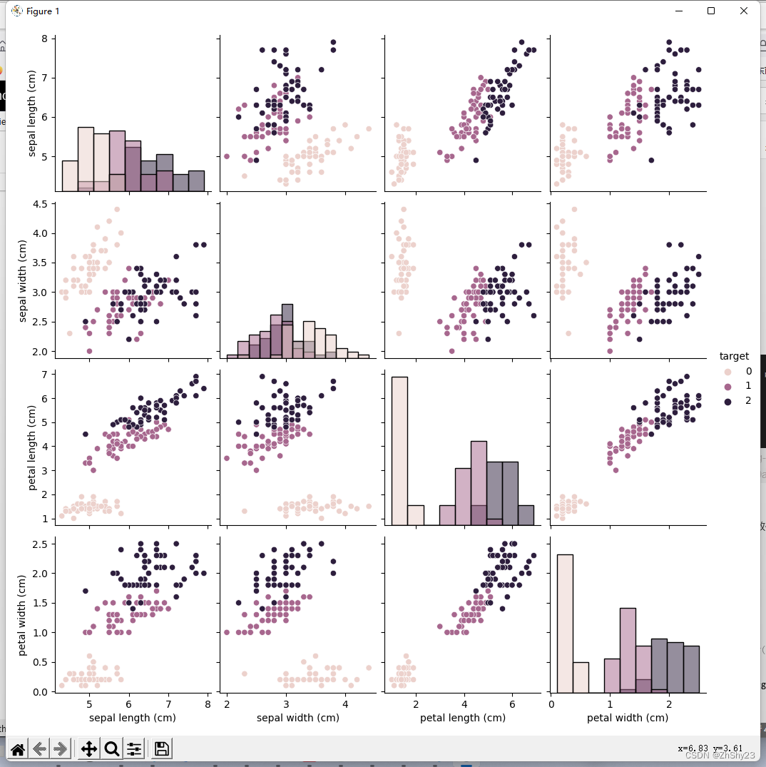 iris_all['target'] = iris_target # 特征与标签组合的散点可视化 sns.pairplot(data=iris_all, diag_kind='hist', hue='target') plt.show() 从上图可以发现,在2D情况下不同的特征组合对于不同类别的花的散点分布,以及大概的区分能力。
for col in iris_features.columns:
    sns.boxplot(x='target', y=col, saturation=0.5,
                palette='pastel', data=iris_all)
    plt.title(col)
    plt.show()


 利用箱型图我们也可以得到不同类别在不同特征上的分布差异情况。
# 选取其前三个特征绘制三维点图
fig = plt.figure(figsize=(10, 8))
ax = fig.add_subplot(111, projection='3d')

iris_all_class0 = iris_all[iris_all['target'] == 0].values
iris_all_class1 = iris_all[iris_all['target'] == 1].values
iris_all_class2 = iris_all[iris_all['target'] == 2].values
# 'setosa'(0), 'versicolor'(1), 'virginica'(2)

ax.scatter(iris_all_class0[:, 0], iris_all_class0[:,
           1], iris_all_class0[:, 2], label='setosa')
ax.scatter(iris_all_class1[:, 0], iris_all_class1[:, 1],
           iris_all_class1[:, 2], label='versicolor')
ax.scatter(iris_all_class2[:, 0], iris_all_class2[:, 1],
           iris_all_class2[:, 2], label='virginica')
plt.legend()

plt.show()
-
利用 逻辑回归模型 在二分类上 进行训练和预测
# 为了正确评估模型性能,将数据划分为训练集和测试集,并在训练集上训练模型,在测试集上验证模型性能。
from sklearn.model_selection import train_test_split

# 选择其类别为0和1的样本 (不包括类别为2的样本)
iris_features_part = iris_features.iloc[:100]
iris_target_part = iris_target[:100]

# 测试集大小为20%, 80%/20%分
x_train, x_test, y_train, y_test = train_test_split(
    iris_features_part, iris_target_part, test_size=0.2, random_state=2020)

## 从sklearn中导入逻辑回归模型
from sklearn.linear_model import LogisticRegression

# 定义 逻辑回归模型
clf = LogisticRegression(random_state=0, solver='lbfgs')

# 在训练集上训练逻辑回归模型
clf.fit(x_train, y_train)

# 查看其对应的w
print('the weight of Logistic Regression:', clf.coef_)

# 查看其对应的w0
print('the intercept(w0) of Logistic Regression:', clf.intercept_)
===============================
the weight of Logistic Regression: [[ 0.45181973 -0.81743611  2.14470304  0.89838607]]
the intercept(w0) of Logistic Regression: [-6.53367714]
================================
# 在训练集和测试集上分布利用训练好的模型进行预测 train_predict = clf.predict(x_train) test_predict = clf.predict(x_test) # 利用accuracy(准确度)【预测正确的样本数目占总预测样本数目的比例】评估模型效果 print('The accuracy of the Logistic Regression is:', metrics.accuracy_score(y_train, train_predict)) print('The accuracy of the Logistic Regression is:', metrics.accuracy_score(y_test, test_predict)) ## 查看混淆矩阵 (预测值和真实值的各类情况统计矩阵) confusion_matrix_result = metrics.confusion_matrix(test_predict, y_test) print('The confusion matrix result:\n', confusion_matrix_result) ======================== The accuracy of the Logistic Regression is: 1.0 The accuracy of the Logistic Regression is: 1.0 The confusion matrix result: [[ 9 0] [ 0 11]]# 利用热力图对于结果进行可视化 plt.figure(figsize=(8, 6)) sns.heatmap(confusion_matrix_result, annot=True, cmap='Blues') plt.xlabel('Predicted labels') plt.ylabel('True labels') plt.show()
-
利用 逻辑回归模型 在三分类(多分类)上 进行训练和预测
# 测试集大小为20%, 80%/20%分
x_train, x_test, y_train, y_test = train_test_split(
    iris_features, iris_target, test_size=0.2, random_state=2020)

# 定义 逻辑回归模型
clf = LogisticRegression(random_state=0, solver='lbfgs')

# 在训练集上训练逻辑回归模型
clf.fit(x_train, y_train)

# 查看其对应的w
print('the weight of Logistic Regression:\n', clf.coef_)

# 查看其对应的w0
print('the intercept(w0) of Logistic Regression:\n', clf.intercept_)

# 由于这个是3分类,所有我们这里得到了三个逻辑回归模型的参数,其三个逻辑回归组合起来即可实现三分类。
============================
the weight of Logistic Regression:
 [[-0.45928925  0.83069886 -2.26606531 -0.99743981]
 [ 0.33117319 -0.72863423 -0.06841147 -0.9871103 ]
 [ 0.12811606 -0.10206463  2.33447678  1.9845501 ]]
the intercept(w0) of Logistic Regression:
 [  9.43880675   3.93047364 -13.36928039]
# 在训练集和测试集上分布利用训练好的模型进行预测 train_predict = clf.predict(x_train) test_predict = clf.predict(x_test) # 由于逻辑回归模型是概率预测模型(前文介绍的 p = p(y=1|x,\theta)),所有我们可以利用 predict_proba 函数预测其概率 train_predict_proba = clf.predict_proba(x_train) test_predict_proba = clf.predict_proba(x_test) print('The test predict Probability of each class:\n', test_predict_proba) # 其中第一列代表预测为0类的概率,第二列代表预测为1类的概率,第三列代表预测为2类的概率。 # 利用accuracy(准确度)【预测正确的样本数目占总预测样本数目的比例】评估模型效果 print('The accuracy of the Logistic Regression is:', metrics.accuracy_score(y_train, train_predict)) print('The accuracy of the Logistic Regression is:', metrics.accuracy_score(y_test, test_predict)) ==================== The test predict Probability of each class: [[1.03461735e-05 2.33279476e-02 9.76661706e-01] [9.69926591e-01 3.00732874e-02 1.21676998e-07] [2.09992548e-02 8.69156617e-01 1.09844128e-01] [3.61934871e-03 7.91979966e-01 2.04400685e-01] [7.90943204e-03 8.00605299e-01 1.91485269e-01] [7.30034958e-04 6.60508053e-01 3.38761912e-01] [1.68614210e-04 1.86322045e-01 8.13509341e-01] [1.06915331e-01 8.90815532e-01 2.26913668e-03] [9.46928071e-01 5.30707292e-02 1.20016058e-06] [9.62346385e-01 3.76532232e-02 3.91897292e-07] [1.19533385e-04 1.38823468e-01 8.61056998e-01] [8.78881882e-03 6.97207360e-01 2.94003821e-01] [9.73938143e-01 2.60617345e-02 1.22613837e-07] [1.78434056e-03 4.79518177e-01 5.18697483e-01] [5.56924343e-04 2.46776841e-01 7.52666235e-01] [9.83549842e-01 1.64500669e-02 9.13617262e-08] [1.65201476e-02 9.54672748e-01 2.88071039e-02] [8.99853712e-03 7.82707576e-01 2.08293887e-01] [2.98015027e-05 5.45900067e-02 9.45380192e-01] [9.35695863e-01 6.43039516e-02 1.85301362e-07] [9.80621190e-01 1.93787400e-02 7.00125252e-08] [1.68478816e-04 3.30167226e-01 6.69664295e-01] [3.54046164e-03 4.02267805e-01 5.94191734e-01] [9.70617284e-01 2.93824739e-02 2.42443968e-07] [2.56895206e-04 1.54631583e-01 8.45111522e-01] [3.48668491e-02 9.11966140e-01 5.31670106e-02] [1.47218847e-02 6.84038114e-01 3.01240001e-01] [9.46510451e-04 4.28641987e-01 5.70411503e-01] [9.64848137e-01 3.51516748e-02 1.87917882e-07] [9.70436779e-01 2.95624024e-02 8.18591611e-07]] The accuracy of the Logistic Regression is: 0.9833333333333333 The accuracy of the Logistic Regression is: 0.8666666666666667# 查看混淆矩阵 confusion_matrix_result = metrics.confusion_matrix(test_predict, y_test) print('The confusion matrix result:\n', confusion_matrix_result) # 利用热力图对于结果进行可视化 plt.figure(figsize=(8, 6)) sns.heatmap(confusion_matrix_result, annot=True, cmap='Blues') plt.xlabel('Predicted labels') plt.ylabel('True labels') plt.show()
通过结果我们可以发现,其在三分类的结果的预测准确度上有所下降,其在测试集上的准确度为: 86.67 % 86.67\% 86.67%,这是由于’versicolor’(1)和 ‘virginica’(2)这两个类别的特征,我们从可视化的时候也可以发现,其特征的边界具有一定的模糊性(边界类别混杂,没有明显区分边界),所有在这两类的预测上出现了一定的错误。


 223
223

 被折叠的 条评论
为什么被折叠?
被折叠的 条评论
为什么被折叠?
 到【灌水乐园】发言


