pytorch常用API和知识点(一)

一、Dataset, DataLoader产生自定义的训练数据

pytorch Dataset, DataLoader产生自定义的训练数据

1. torch.utils.data.Dataset

datasets这是一个pytorch定义的dataset的源码集合。下面是一个自定义Datasets的基本框架，初始化放在__init__()中，其中__getitem__()和__len__()两个方法是必须重写的。getitem()返回训练数据，如图片和label，而__len__()返回数据长度。

class CustomDataset(data.Dataset):#需要继承data.Dataset
    def __init__(self):
        # TODO
        # 1. Initialize file path or list of file names.
        pass
    def __getitem__(self, index):
        # TODO
        # 1. Read one data from file (e.g. using numpy.fromfile, PIL.Image.open).
        # 2. Preprocess the data (e.g. torchvision.Transform).
        # 3. Return a data pair (e.g. image and label).
        #这里需要注意的是，第一步：read one data，是一个data
        pass
    def __len__(self):
        # You should change 0 to the total size of your dataset.
        return 0

2. torch.utils.data.DataLoader

DataLoader(object)可用参数：
torch.utils.data.DataLoader(
    dataset,
    batch_size=1,
    shuffle=False,
    sampler=None,
    batch_sampler=None, 
    num_workers=0,
    collate_fn=None, 
    pin_memory=False, 
    drop_last=False,
    timeout=0, 
    worker_init_fn=None,
    multiprocessing_context=None)
  

dataset(Dataset): 传入的数据集
batch_size(int, optional): 每个batch有多少个样本
shuffle(bool, optional): 在每个epoch开始的时候，对数据进行重新排序
sampler(Sampler, optional): 自定义从数据集中取样本的策略，如果指定这个参数，那么shuffle必须为False
batch_sampler(Sampler, optional): 与sampler类似，但是一次只返回一个batch的indices（索引），需要注意的是，一旦指定了这个参数，那么batch_size,shuffle,sampler,drop_last就不能再制定了（互斥——Mutually exclusive）
num_workers (int, optional): 这个参数决定了有几个进程来处理data loading。0意味着所有的数据都会被load进主进程。（默认为0）
collate_fn (callable, optional): 将一个list的sample组成一个mini-batch的函数
pin_memory (bool, optional)： 如果设置为True，那么data loader将会在返回它们之前，将tensors拷贝到CUDA中的固定内存（CUDA pinned memory）中.
drop_last (bool, optional):如果设置为True：这个是对最后的未完成的batch来说的，比如你的batch_size设置为64，而一个epoch只有100个样本，那么训练的时候后面的36个就被扔掉了。 
    	如果为False（默认），那么会继续正常执行，只是最后的batch_size会小一点。
timeout(numeric, optional):如果是正数，表明等待从worker进程中收集一个batch等待的时间，若超出设定的时间还没有收集到，那就不收集这个内容了。这个numeric应总是大于等于0。默认为0
worker_init_fn (callable, optional): 每个worker初始化函数 If not None, this will be called on eachworker subprocess with the worker id (an int in [0, num_workers - 1]) as input, 
    	after seeding and before data loading. (default: None) 
      Epoch, Iteration, Batchsize
    Epoch: 所有训练样本都已经输入到模型中，称为一个 Epoch
    Iteration: 一批样本输入到模型中，称为一个 Iteration
    Batchsize: 批大小，决定一个 iteration 有多少样本，也决定了一个 Epoch 有多少个 Iteration     

二、torch相关模块

1.导入相关模块

from __future__ import print_function
import os
import torch
import torch.nn as nn
import torch.nn.functional as F
import torch.optim as optim
from torch.autograd import Variable

from torch.utils.data import Dataset
from torch.utils.data import DataLoader

import torchvision
from torchvision import datasets
from torchvision import transforms
from torchvision import utils
import matplotlib.pyplot as plt
import numpy as np

#忽略警告

import warnings
warnings.filterwarnings("ignore")

2. 利用内置数据集构建神经网络并训练

pytorch 中文文档

import torch
import torchvision
import torchvision.transforms as transforms
import torch.nn as nn
import torch.nn.functional as F
import torch.optim as optim

#torchvision 数据集的输出是范围在[0,1]之间的 PILImage，我们将他们转换成归一化范围为[-1,1]之间的张量 Tensors。
transform = transforms.Compose(
    	[transforms.ToTensor(),transforms.Normalize((0.5, 0.5, 0.5), (0.5, 0.5, 0.5))])
trainset = torchvision.datasets.CIFAR10(root='./data', train=True,download=True, transform=transform)
testset = torchvision.datasets.CIFAR10(root='./data', train=False, download=True, transform=transform)
trainloader = torch.utils.data.DataLoader(trainset, batch_size=4,shuffle=True,  num_workers=2)
testloader  = torch.utils.data.DataLoader(testset,  batch_size=4,shuffle=False, num_workers=2)
classes = ('plane', 'car', 'bird', 'cat','deer', 'dog', 'frog', 'horse', 'ship', 'truck')
#定义一个卷积神经网络 在这之前先 从神经网络章节 复制神经网络，并修改它为3通道的图片(在此之前它被定义为1通道)

class Net(nn.Module):
    def __init__(self):
        super(Net, self).__init__()
        self.conv1 = nn.Conv2d(3, 6, 5)
        self.pool = nn.MaxPool2d(2, 2)
        self.conv2 = nn.Conv2d(6, 16, 5)
        self.fc1 = nn.Linear(16 * 5 * 5, 120)
        self.fc2 = nn.Linear(120, 84)
        self.fc3 = nn.Linear(84, 10)
        
    def forward(self, x):
        x = self.pool(F.relu(self.conv1(x)))
        x = self.pool(F.relu(self.conv2(x)))
        x = x.view(-1, 16 * 5 * 5)
        x = F.relu(self.fc1(x))
        x = F.relu(self.fc2(x))
        x = self.fc3(x)
        return x

net = Net()
criterion = nn.CrossEntropyLoss()
optimizer = optim.SGD(net.parameters(), lr=0.001, momentum=0.9)

#训练网络 这里事情开始变得有趣，我们只需要在数据迭代器上循环传给网络和优化器 输入就可以。
for epoch in range(2):  # loop over the dataset multiple times
    running_loss = 0.0
    for i, data in enumerate(trainloader, 0):
        # get the inputs
        inputs, labels = data
        # zero the parameter gradients
        optimizer.zero_grad()
        
        # forward + backward + optimize
        outputs = net(inputs)
        loss = criterion(outputs, labels)
        loss.backward()
        optimizer.step()

        # print statistics
        running_loss += loss.item()
        if i % 2000 == 1999:    # print every 2000 mini-batches
            print('[%d, %5d] loss: %.3f' %
                  (epoch + 1, i + 1, running_loss / 2000))
            running_loss = 0.0

print('Finished Training')
outputs = net(images)
#输出是预测与十个类的近似程度，与某一个类的近似程度越高，网络就越认为图像是属于这一类别。所以让我们打印其中最相似类别类标：
_, predicted = torch.max(outputs, 1)
print('Predicted: ', ' '.join('%5s' % classes[predicted[j]] for j in range(4)))2-1

3.torchvision

PyTorch 学习笔记
我们在安装PyTorch时，还安装了torchvision，这是一个计算机视觉工具包。有 3 个主要的模块：torchvision.transforms 里面包括常用的图像预处理方法
torchvision.datasets 里面包括常用数据集如 mnist、CIFAR-10、Image-Net 等
torchvision.models 里面包括常用的预训练好的模型，如 AlexNet、VGG、ResNet、GoogleNet 等
深度学习模型是由数据驱动的，数据的数量和分布对模型训练的结果起到决定性作用。所以我们需要对数据进行预处理和数据增强。
下面是用数据增强，从一张图片经过各种变换生成 64 张图片，增加了数据的多样性，这可以提高模型的泛化能力。
常用的图像预处理方法有：

• 数据中心化
• 数据标准化
• 缩放
• 裁剪
• 旋转
• 翻转
• 填充
• 噪声添加
• 灰度变换
• 线性变换
• 仿射变换 亮度、饱和度以及对比度变换

4.torchvision.transforms

ToTensor类是实现：Convert a PIL Image or numpy.ndarray to tensor的过程，在PyTorch中常用PIL库来读取图像数据，因此这个方法相当于搭建了PILImage和Tensor的桥梁
另外要强调的是在做数据归一化之前必须要把PILImage转成Tensor，而其他resize或crop操作则不需要。

self.data_transforms = {
    'train': transforms.Compose([
        transforms.Resize(84),
        transforms.CenterCrop(84),
        # 转换成tensor向量
        transforms.ToTensor(),
        # 对图像进行归一化操作
        # [0.485, 0.456, 0.406]，RGB通道的均值与标准差
        transforms.Normalize([0.485, 0.456, 0.406], [0.229, 0.224, 0.225])
    ]),
    'test': transforms.Compose([
        transforms.Resize(84),
        transforms.CenterCrop(84),
        transforms.ToTensor(),
        transforms.Normalize([0.485, 0.456, 0.406], [0.229, 0.224, 0.225])
    ]),
}
train_dataset = my_Data_Set('./train.txt', root_Dir=trainData_path, transform=self.data_transforms['train'])
train_loader = DataLoader(train_dataset, batch_size=batch_size, shuffle=True)

5.定义神经网络

import torch
import torch.nn as nn
import torch.nn.functional as F


class Net(nn.Module):

    def __init__(self):
        super(Net, self).__init__()
        # 1 input image channel, 6 output channels, 5x5 square convolution
        # kernel
        self.conv1 = nn.Conv2d(1, 6, 5)
        self.conv2 = nn.Conv2d(6, 16, 5)
        # an affine operation: y = Wx + b
        self.fc1 = nn.Linear(16 * 5 * 5, 120)
        self.fc2 = nn.Linear(120, 84)
        self.fc3 = nn.Linear(84, 10)

    def forward(self, x):
        # Max pooling over a (2, 2) window
        x = F.max_pool2d(F.relu(self.conv1(x)), (2, 2))
        # If the size is a square you can only specify a single number
        x = F.max_pool2d(F.relu(self.conv2(x)), 2)
        x = x.view(-1, self.num_flat_features(x))
        x = F.relu(self.fc1(x))
        x = F.relu(self.fc2(x))
        x = self.fc3(x)
        return x

    def num_flat_features(self, x):
        size = x.size()[1:]  # all dimensions except the batch dimension
        num_features = 1
        for s in size:
            num_features *= s
        return num_features
net = Net()
print(net)

输出：
Net(
  (conv1): Conv2d(1, 6, kernel_size=(5, 5), stride=(1, 1))
  (conv2): Conv2d(6, 16, kernel_size=(5, 5), stride=(1, 1))
  (fc1): Linear(in_features=400, out_features=120, bias=True)
  (fc2): Linear(in_features=120, out_features=84, bias=True)
  (fc3): Linear(in_features=84, out_features=10, bias=True)
)

三、Tensor相关运算

1.创建tensor

import torch
a=torch.ones(2,3)
a=torch.ones_like(2,3)
a=torch.zeros(2,3)
a=torch.zeros_like(2,3)
a=torch.eye(3,3)  #斜对角为1
a=torch.range(1,9,2) 
a=torch.linspace(1,9,3) #1-9之间等间隔3个数
d = torch.empty(2,3)
torch.rand(sizes, out=None)     #产生一个服从均匀分布的张量，张量内的数据包含从区间[0,1)的随机数。参数size是一个整数序列，用于定义张量大小
torch.randn(sizes, out=None)    #产生一个服从标准整正态分布的张量，张量内数据均值为0，方差为1，即为高斯白噪声。sizes作用同上。
torch.randint(low=0, high, size, out=None, requires_grad=False)   #返回一个张量，该张量填充了在[low,high)均匀生成的随机整数。张量的形状由可变的参数大小定义。
-->torch.LongTensor
torch.normal(means, std, out=None)  #产生一个服从离散正态分布的张量随机数，可以指定均值和标准差。其中，标准差std是一个张量包含每个输出元素相关的正态分布标准差。
torch.randperm(n, out=None, requires_grad=True)  #返回从0到n-1的整数的随机排列数
-->#tensor([2, 3, 1, 0, 4]) -->torch.LongTensor

2.加减乘除,乘方,矩阵乘法,对数指数

import torch
##add
a = torch.rand(2, 3)
b = torch.rand(2, 3)

print(a + b)
print(torch.add(a, b))
print(a.add(b))
print(a.add_(b))

#sub
print("==== sub res ====")
print(a - b)
print(torch.sub(a, b))
print(a.sub(b))
print(a.sub_(b))

## mul #对应位置元素相乘
print("===== mul ====")
print(a * b)
print(torch.mul(a, b))
print(a.mul(b))
print(a.mul_(b))

# div  #对应位置元素相除
print("=== div ===")
print(a/b)
print(torch.div(a, b))
print(a.div(b))
print(a.div_(b))

###matmul  矩阵乘法
a = torch.ones(2, 1)
b = torch.ones(1, 2)
print(a @ b)
print(a.matmul(b))
print(torch.matmul(a, b))
print(torch.mm(a, b))
print(a.mm(b))

##高维tensor dim>2 ,定义其矩阵乘法仅在最后两个维度上,前面的唯独必须保持一致,就像矩阵的索引一样,并且操作只有torch.matmul()
a = torch.ones(1, 2, 3, 4)
b = torch.ones(1, 2, 4, 3)
print(a.matmul(b).shape)

##pow 乘方
a = torch.tensor([1, 2])
print(a**3)
print(torch.pow(a, 3))
print(a.pow(3))
print(a.pow_(3))

#exp
a = torch.tensor([1, 2], dtype=torch.float32)
print(a.type())
print(torch.exp(a))
print(torch.exp_(a))
print(a.exp())
print(a.exp_())

##log
a = torch.tensor([10, 2],dtype=torch.float32)
print(torch.log(a))
print(torch.log_(a))
print(a.log())
print(a.log_())

##sqrt  开平方
a = torch.tensor([10, 2],dtype=torch.float32)
print(torch.sqrt(a))
print(torch.sqrt_(a))
print(a.sqrt())
print(a.sqrt_())



3.取整取余运算
import torch
a = torch.rand(2, 2)
a = a * 10
print(a)

print(torch.floor(a))	#向下取整
print(torch.ceil(a))	#向上取整
print(torch.round(a))	#四舍五入 >=0.5向上取整,<0.5向下取整
print(torch.trunc(a))     #裁剪,只取整数部分
print(torch.frac(a))      #裁剪,只取小数部分
print(a % 2)		#取余数
b = torch.tensor([[2, 3], [4, 5]],dtype=torch.float)
print (a, b))
print(torch.remainder(a, b))

4. 比较排序运算

print(torch.eq(a, b))     #逐个元素比较,返回逐个元素位置比较结果
print(torch.equal(a, b))  #如果a b 有相同唯独和elements,返回一个布尔值True
print(torch.ge(a, b))	#a>=b
print(torch.gt(a, b))	#a>b
print(torch.le(a, b))	#a<=b
print(torch.lt(a, b))	#a<b
print(torch.ne(a, b))	#a!=b
#沿给定dim维度返回输入张量input中k个最大值，不指定dim，
则默认为最后一维，如果largest为False，则返回最小的k个值。
torch.topk(input, k, dim=None, largest=True, sorted=True, out=None)

#取input指定维度上第k个最小值，若不指定dim，则默认为input的最后一维。返回一个元组，其中indices是原始输入张量input中沿dim维的第k个最小值下标
torch.kthvalue(input, k, dim=None, out=None) 

#对输入张量input沿着指定维度按升序排序，如果不给定dim，默认为输入的最后一维。如果指定参数descending为True，则按降序排序。
返回两项：重排后的张量，和重排后元素在原张量的索引
 torch.sort(input, dim=None, descending=False, out=None) -> (Tensor, LongTensor):

5.numpy的ndarray 和tensor相互转换

Tensor on GPU
import numpy as np
import cv2

data = cv2.imread("test.png")
cv2.imshow("test1", data)
# cv2.waitKey(0)
dev_cpu=torch.device("cpu") #torch.device代表将torch.Tensor分配到的设备的对象。
dev_gpu=torch.device("cuda")
# a = np.zeros([2, 2])
out = torch.from_numpy(data) #从numpy   转化为Tensor
out = out.to(dev_gpu)  #用方法to可以将tensor 在cpu 和gpu(需要硬件支持)之间相互移动
print(out.is_cuda)

out = torch.flip(out, dims=[0])
out = out.to(dev_cpu)
print(out.is_cuda)
data = out.numpy()

6.多设备,并行和分布式

cuda 相关

import torch
torch.cuda.is_available()     #检查cuda是否可以使用  device = torch.device("cuda:0" if torch.cuda.is_available() else "cpu")
torch.cuda.current_device()            #查看当前gpu索引号
torch.cuda.current_stream(device=0)          #查看当前cuda流
torch.cuda.device(1)        #选择device
torch.cuda.device_count()         #查看有多少个GPU设备
torch.cuda.get_device_capability(device=0) #查看gpu的容量

并行化 Parallelism

torch.get_num_threads():	  #获得用于并行化CPU操作的OpenMP线程数
torch.set_num_threads(int):  #设定用于并行化CPU操作的OpenMP线程数

CPU GPU 之间转换

dev_cpu=torch.device("cpu") #torch.device代表将torch.Tensor分配到的设备的对象。
dev_gpu=torch.device("cuda")
#data = np.zeros([2, 2])
out = torch.from_numpy(data) #从numpy   转化为Tensor
out = out.to(dev_gpu)  #用方法to可以将tensor 在cpu 和gpu(需要硬件支持)之间相互移动

7.PyTorch 中常见的基础型张量操作 .numpy()、.item()、.detach()、.gpu()、.cpu()

.numpy()
官方文档：https://pytorch.org/docs/stable/tensors.html#torch.Tensor.numpy
功能：将张量转换为与其共享底层存储的 n 维 numpy 数组

.item()
官方文档：https://pytorch.org/docs/stable/tensors.html#torch.Tensor.cpu
功能：将张量的值转换为标准的 Python 数值，只有当张量仅含一个元素时才能使用它

.detach()
官方文档：https://pytorch.org/docs/stable/autograd.html#torch.Tensor.detach
功能：返回一个与当前 graph 分离的、不再需要梯度的新张量

.cuda()
官方文档：https://pytorch.org/docs/stable/tensors.html#torch.Tensor.cuda
功能：将张量拷贝到 GPU 上

.cpu()
官方文档：https://pytorch.org/docs/stable/tensors.html#torch.Tensor.cpu
功能：将张量拷贝到 CPU 上

8.x[:,:,None,:]

None相当于在数组中多加一个维度
import numpy as np
x = np.arange(24).reshape((2,3,4))
print(x.shape)  #(2,3,4)
x1= x[:,:,None,:] #(2, 3, 1, 4)
x2=x[:,:,:,None] #(2, 3, 4, 1)
print(x1.shape)
print(x2.shape)
x3=x1-x2 #这里相减时用到了广播机制，都先变成(2,3,4,4),再相减 输出，形状(2,3,4,4)：
#print(x3)
print(x3.shape) #(2, 3, 4, 4)

四、相关函数介绍

1.上下采样插值函数torch.nn.functional.interpolate

torch.nn.functional.interpolate(input, size=None, scale_factor=None, mode=‘nearest’, align_corners=None)
这个函数是用来上采样或下采样，可以给定size或者scale_factor来进行上下采样。同时支持3D、4D、5D的张量输入。
插值算法可选，最近邻、线性、双线性等等。
图像的五种插值算法

#参数介绍
input (Tensor) – the input tensor
size (int or Tuple[int] or Tuple[int, int] or Tuple[int, int, int]) – output spatial size.
scale_factor (float or Tuple[float]) – multiplier for spatial size. Has to match input size if it is a tuple.
mode (str) – algorithm used for upsampling: 'nearest' 最近邻| 'linear' 线性| 'bilinear' 双线性| 'bicubic' 双三次插值算法 |'trilinear' 三线性| 'area'. Default: 'nearest'
align_corners (bool, optional) – Geometrically, we consider the pixels of the input and output as squares rather than points. 
    If set to True, the input and output tensors are aligned by the center points of their corner pixels, preserving the values at the corner pixels.
    If set to False, the input and output tensors are aligned by the corner points of their corner pixels, and the interpolation uses edge value padding for out-of-boundary 
    values, making this operation independent of input size when scale_factor is kept the same. 
    This only has an effect when mode is 'linear', 'bilinear', 'bicubic' or 'trilinear'. Default: False

2.pytorch torch.nn 实现上采样——nn.Upsample

CLASS torch.nn.Upsample(size=None, scale_factor=None, mode='nearest', align_corners=None)

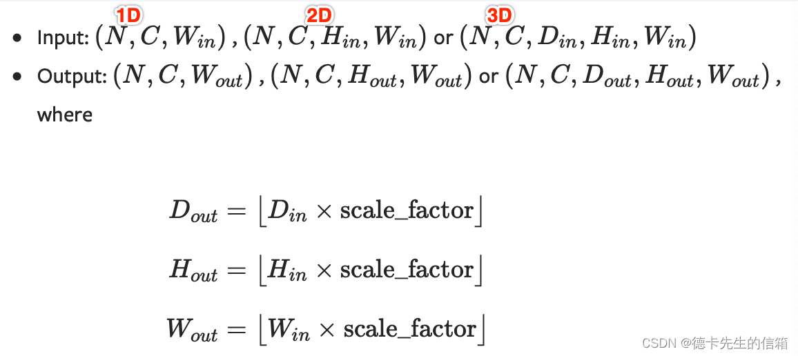
上采样一个给定的多通道的 1D (temporal,如向量数据), 2D (spatial，如jpg、png等图像数据) or 3D (volumetric，如点云数据)
数据假设输入数据的格式为minibatch x channels x [optional depth] x [optional height] x width。
因此对于一个空间spatial输入，我们期待着4D张量的输入，即minibatch x channels x height x width。
而对于体积volumetric输入，我们则期待着5D张量的输入，即minibatch x channels x depth x height x width
对于上采样有效的算法分别有对 3D, 4D和 5D 张量输入起作用的 最近邻、线性,、双线性, 双三次(bicubic)和三线性(trilinear)插值算法
你可以给定scale_factor来指定输出为输入的scale_factor倍或直接使用参数size指定目标输出的大小（但是不能同时制定两个）

参数：
size (int or Tuple[int] or Tuple[int, int] or Tuple[int, int, int], optional) – 根据不同的输入类型制定的输出大小
scale_factor (float or Tuple[float] or Tuple[float, float] or Tuple[float, float, float], optional) – 指定输出为输入的多少倍数。如果输入为tuple，其也要制定为tuple类型
mode (str, optional) – 可使用的上采样算法，有'nearest', 'linear', 'bilinear', 'bicubic' and 'trilinear'. 默认使用'nearest'
align_corners (bool, optional) – 如果为True，输入的角像素将与输出张量对齐，因此将保存下来这些像素的值。仅当使用的算法为'linear', 'bilinear'or 'trilinear'时可以使用。默认设置为False

输入输出形状：

注意：
当align_corners = True时，线性插值模式(线性、双线性、双三线性和三线性)不按比例对齐输出和输入像素，因此输出值可以依赖于输入的大小。
这是0.3.1版本之前这些模式的默认行为。从那时起，默认行为是align_corners = False,如下图：

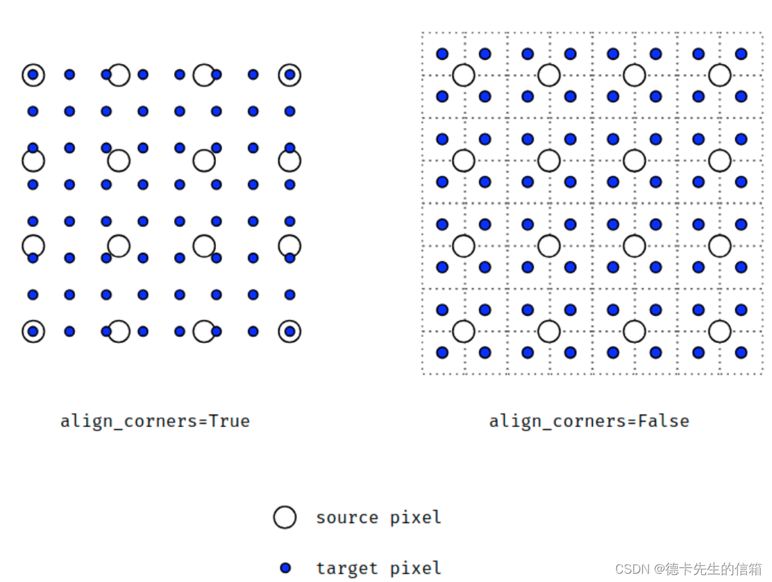
上面的图是source pixel为44上采样为target pixel为88的两种情况，这就是对齐和不对齐的差别，会对齐左上角元素，即设置为align_corners = True时输入的左上角元素是一定等于输出的左上角元素。但是有时align_corners = False时左上角元素也会相等，官网上给的例子就不太能说明两者的不同(也没有试出不同的例子，大家理解这个概念就行了)
如果您想下采样/常规调整大小，您应该使用interpolate()方法，这里的上采样方法已经不推荐使用了。

3.torch.clamp

将输入input张量每个元素的夹紧到区间 [min,max][min,max]，并返回结果到一个新张量。
torch.clamp(input, min, max, out=None) → Tensor
| min, if x_i < min
y_i = | x_i, if min <= x_i <= max
| max, if x_i > max

参数：
input (Tensor) – 输入张量
min (Number) – 限制范围下限
max (Number) – 限制范围上限
out (Tensor, optional) – 输出张量

代码示例如下:
a=torch.randint(low=0,high=10,size=(10,1))
print(a)
a=torch.clamp(a,3,9)
print(a)
tensor([[9.],[3.],[0.],[4.],[4.],[2.], [4.],[1.],[2.],[9.]])
tensor([[9.],[3.],[3.],[4.],[4.],[3.], [4.],[3.],[3.],[9.]])

关于with torch.no_grad():
在使用pytorch时，并不是所有的操作都需要进行计算图的生成（计算过程的构建，以便梯度反向传播等操作）。而对于tensor的计算操作，默认是要进行计算图的构建的，在这种情况下，可以使用 with torch.no_grad():，强制之后的内容不进行计算图构建。

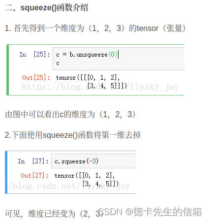
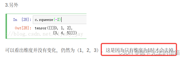
4.torch.unsqueeze 详解

unsqueeze() 扩展维度 返回一个新的张量，对输入的既定位置插入维度 1
注意：
返回张量与输入张量共享内存，所以改变其中一个的内容会改变另一个。
参数:
tensor (Tensor) – 输入张量
dim (int)– 插入维度的索引
out (Tensor, optional)–结果张量

5.torch.cat()

#cat是concatnate的意思：拼接，联系在一起
C = torch.cat( (A,B),0 )  #按维数0拼接（竖着拼）
C = torch.cat( (A,B),1 )  #按维数1拼接（横着拼）
>>> import torch
>>> A=torch.ones(2,3)    #2x3的张量（矩阵）                                     
>>> A
tensor([[ 1.,  1.,  1.],
        [ 1.,  1.,  1.]])
>>> B=2*torch.ones(4,3)  #4x3的张量（矩阵）                                    
>>> B
tensor([[ 2.,  2.,  2.],
        [ 2.,  2.,  2.],
        [ 2.,  2.,  2.],
        [ 2.,  2.,  2.]])
>>> C=torch.cat((A,B),0)  #按维数0（行）拼接
>>> C
tensor([[ 1.,  1.,  1.],
         [ 1.,  1.,  1.],
         [ 2.,  2.,  2.],
         [ 2.,  2.,  2.],
         [ 2.,  2.,  2.],
         [ 2.,  2.,  2.]])
>>> C.size()
torch.Size([6, 3])
>>> D=2*torch.ones(2,4) #2x4的张量（矩阵）
>>> C=torch.cat((A,D),1)#按维数1（列）拼接
>>> C
tensor([[ 1.,  1.,  1.,  2.,  2.,  2.,  2.],
        [ 1.,  1.,  1.,  2.,  2.,  2.,  2.]])
>>> C.size()
torch.Size([2, 7])

6.模型保存与恢复

把原先模型eval，把加载后模型eval。才保证两模型完全一样。
加载后不同
如果不指定模型eval模式，那么加载回来的模型并不是和原先保存的模型相同。
简单说，原先的net你要eval一下，load之后的net也要eval一下，把所有参数freeze掉。才保证两个net完全相同（输入相同tensor得到完全一致的结果）。

#保存

net=net.eval()
torch.save(net,'./model.pth')
torch.save(net.state_dict(),'./model-dict.pth')

#加载

net_load1=torch.load('./model.pth')
net_load1=net_load1.eval()

net_load2.load_state_dict(torch.load('./model-dict.pth'))
net_load2=net_load2.eval()

#此时net和net_load1、net_load2完全一样。

7.torch.nn.conv3d理解

class torch.nn.Conv3d(in_channels, out_channels, kernel_size, stride=1, padding=0, dilation=1, groups=1, bias=True)

参数介绍

in_channels(int) – 输入信号的通道，就是输入中每帧图像的通道数
out_channels(int) – 卷积产生的通道，就是输出中每帧图像的通道数
kernel_size(int or tuple) - 过滤器的尺寸，假设为(a,b,c)，表示的是过滤器每次处理 a 帧图像，该图像的大小是b x c。
stride(int or tuple, optional) - 卷积步长，形状是三维的，假设为(x,y,z)，表示的是三维上的步长是x，在行方向上步长是y，在列方向上步长是z。
padding(int or tuple, optional) - 输入的每一条边补充0的层数，形状是三维的，假设是(l,m,n)，表示的是在输入的三维方向前后分别padding l 个全零二维矩阵，在输入的行方向上下分别padding m 个全零行向量，在输入的列方向左右分别padding n 个全零列向量。
dilation(int or tuple, optional) – 卷积核元素之间的间距，这个看看空洞卷积就okay了
groups(int, optional) – 从输入通道到输出通道的阻塞连接数；没用到，没细看
bias(bool, optional) - 如果bias=True，添加偏置；没用到，没细看
#3D  图像事假要输入5为数据(B,C,D,H,W)
（1，3，7，60，40）表示输入1个视频，每个视频中图像的通道数是3，每个视频中包含的图像数是7，图像的大小是60 x 40。
（3，3，（3，7，7））表示的是输入图像的通道数是3，输出图像的通道数是3，（3，7，7）表示过滤器每次处理3帧图像，卷积核的大小是7 x 7。
stride=1 表示stride=（1，1，1），在三维方向上步长是1，在宽和高上步长也是1。
padding=0 表示padding=（0，0，0）表示在三维方向上不padding，在宽和高上也不padding。

8.torch.meshgrid()和np.meshgrid()的区别

np.meshgrid()函数常用于生成二维网格，比如图像的坐标点。
pytorch中也有一个类似的函数torch.meshgrid()，功能也类似，但是两者的用法有区别，使用时需要注意（刚踩坑，因此记录一下。。。）

比如我要生成一张图像(h=6, w=10)的xy坐标点，看下两者的实现方式：

np.meshgrid()
>>> import numpy as np
>>> h = 6
>>> w = 10
>>> xs, ys = np.meshgrid(np.arange(w), np.arange(h))#差异点y,x
>>> xs.shape
(6, 10)
>>> ys.shape
(6, 10)
>>> xs
array([[0, 1, 2, 3, 4, 5, 6, 7, 8, 9],
       [0, 1, 2, 3, 4, 5, 6, 7, 8, 9],
       [0, 1, 2, 3, 4, 5, 6, 7, 8, 9],
       [0, 1, 2, 3, 4, 5, 6, 7, 8, 9],
       [0, 1, 2, 3, 4, 5, 6, 7, 8, 9],
       [0, 1, 2, 3, 4, 5, 6, 7, 8, 9]])
>>> ys
array([[0, 0, 0, 0, 0, 0, 0, 0, 0, 0],
       [1, 1, 1, 1, 1, 1, 1, 1, 1, 1],
       [2, 2, 2, 2, 2, 2, 2, 2, 2, 2],
       [3, 3, 3, 3, 3, 3, 3, 3, 3, 3],
       [4, 4, 4, 4, 4, 4, 4, 4, 4, 4],
       [5, 5, 5, 5, 5, 5, 5, 5, 5, 5]])
>>> xys = np.stack([xs, ys], axis=-1)
>>> xys.shape
(6, 10, 2)

torch.meshgrid()

>>> import torch
>>> h = 6
>>> w = 10
>>> ys,xs = torch.meshgrid(torch.arange(h), torch.arange(w)) #差异点x,y
>>> xs.shape
torch.Size([6, 10])
>>> ys.shape
torch.Size([6, 10])
>>> xs
tensor([[0, 1, 2, 3, 4, 5, 6, 7, 8, 9],
        [0, 1, 2, 3, 4, 5, 6, 7, 8, 9],
        [0, 1, 2, 3, 4, 5, 6, 7, 8, 9],
        [0, 1, 2, 3, 4, 5, 6, 7, 8, 9],
        [0, 1, 2, 3, 4, 5, 6, 7, 8, 9],
        [0, 1, 2, 3, 4, 5, 6, 7, 8, 9]])
>>> ys
tensor([[0, 0, 0, 0, 0, 0, 0, 0, 0, 0],
        [1, 1, 1, 1, 1, 1, 1, 1, 1, 1],
        [2, 2, 2, 2, 2, 2, 2, 2, 2, 2],
        [3, 3, 3, 3, 3, 3, 3, 3, 3, 3],
        [4, 4, 4, 4, 4, 4, 4, 4, 4, 4],
        [5, 5, 5, 5, 5, 5, 5, 5, 5, 5]])
>>> xys = torch.stack([xs, ys], dim=-1)
>>> xys.shape
torch.Size([6, 10, 2])

9.torch.filp()

torch.flip(input,dim):第一个参数是输入，第二个参数是输入的第几维度，按照维度对输入进行翻转

import torch
x = torch.arange(16).view(2, 2, 2,2)
print('x=\n',x)
a = torch.flip(x, [2])
print('a=\n',a)
x=tensor([[[[ 0,  1],
          [ 2,  3]],
         [[ 4,  5],
          [ 6,  7]]],
        [[[ 8,  9],
          [10, 11]],
         [[12, 13],
          [14, 15]]]])
          
a=tensor([[[[ 2,  3],
          [ 0,  1]],
         [[ 6,  7],
          [ 4,  5]]],
        [[[10, 11],
          [ 8,  9]],
         [[14, 15],
          [12, 13]]]])
 

10.GAP 和GMP

Global Average Pooling(简称GAP，全局池化层)技术最早提出是在这篇论文（第3.2节）中，被认为是可以替代全连接层的一种新技术。
在keras发布的经典模型中，可以看到不少模型甚至抛弃了全连接层，转而使用GAP，
而在支持迁移学习方面，各个模型几乎都支持使用Global Average Pooling和Global Max Pooling(GMP)。 然而，GAP是否真的可以取代全连接层？其背后的原理何在呢？本文来一探究竟。

简而言之，就是在倒数第二层进行改进（用GAP替代FC），使用GAP将倒数第三层的输出转化成特征值。
由此，在网上找了一些GAP的介绍，此处转载一篇还可以的博客：Global average Pooling
Global Average Pooling
这个概念出自于 network in network 。主要是用来解决全连接的问题，其主要是是将最后一层的特征图进行整张图的一个均值池化，形成一个特征点，将这些特征点组成最后的特征向量，进行softmax中进行计算。
举个例子。假如，最后的一层的数据是10个66的特征图，global average pooling是将每一张特征图计算所有像素点的均值，输出一个数据值，这样10 个特征图就会输出10个数据点，将这些数据点组成一个110的向量的话，就成为一个特征向量，就可以送入到softmax的分类中计算了。

self.gap = nn.AdaptiveAvgPool3d(output_size=1)
self.gap = nn.AdaptiveAvgPool3d(output_size=(1,2,3)))

GAP和GMP都是将参数的数量进行缩减，这样一方面可以避免过拟合，另一方面这也更符合CNN的工作结构，把每个feature map和类别输出进行了关联，而不是feature map的unit直接和类别输出进行关联。
差别在于，GMP只取每个feature map中的最重要的region，这样会导致，一个feature map中哪怕只有一个region是和某个类相关的，这个feature map都会对最终的预测产生很大的影响。而GAP则是每个region都进行了考虑，这样可以保证不会被一两个很特殊的region干扰。这篇论文有更详细的说明。

五、损失函数

1.Pytorch详解BCELoss和BCEWithLogitsLoss

 [https://blog.csdn.net/qq_22210253/article/details/85222093](https://blog.csdn.net/qq_22210253/article/details/85222093)

2.基于深度学习的自然图像和医学图像分割：

损失函数设计(1) https://zhuanlan.zhihu.com/p/106005484
损失函数设计(2) https://zhuanlan.zhihu.com/p/106660186

六、Pytorch中的学习率调整方法

注意
对学习率的更新都是在其step()函数被调用以后完成的，这个step表达的含义可以是一次迭代，当然更多情况下应该是一个epoch以后进行一次scheduler.step()，这根据具体问题来确定。此外，根据pytorch官网上给出的说明，scheduler.step()函数的调用应该在训练代码以后：

scheduler = ...
for epoch in range(100):
    train(...)
    validate(...)
    scheduler.step()

————————————————

Pytorch中的学习率调整方法

1. 手动调整optimizer中的lr参数

2. 利用lr_scheduler()提供的几种调整函数

2.1 LambdaLR(自定义函数)

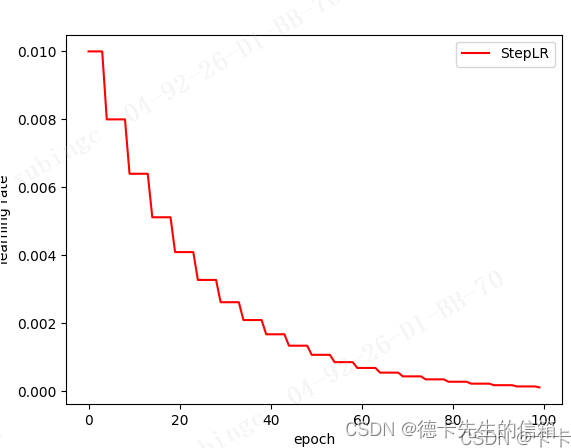
2.2 StepLR(固定步长衰减)

每个step_size步长后使每个参数组的学习率乘上gamma
torch.optim.lr_scheduler.StepLR(optimizer, step_size, gamma=0.1, last_epoch=-1)
optimizer：封装的优化器
step_size： 学习率衰减的周期
gamma：学习率衰减的乘数因子，默认为0.1
last_epoch：最后一个迭代epoch的索引，默认为-1

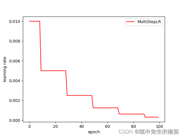
2.3 MultiStepLR(多步长衰减)

当迭代数epoch达到设定值时，每个参数组的学习率将被gamma衰减，这种衰减方式也是在学术论文中最常见的方式，一般手动调整也会采用这种方法

torch.optim.lr_scheduler.MultiStepLR(optimizer, milestones, gamma=0.1, last_epoch=-1)

optimizer：封装的优化器
milestones： 迭代epochs指数列表. 列表中的值必须是增长的
gamma：学习率衰减的乘数因子，默认为0.1
last_epoch：最后一个迭代epoch的索引，默认为-1

其他代码与LambdaLR中相同
#在指定的epoch值，如[10,30,50,70,90]处对学习率进行衰减，lr = lr * gamma
scheduler = lr_scheduler.MultiStepLR(optimizer, milestones=[10,30,50,70,90], gamma=0.5)

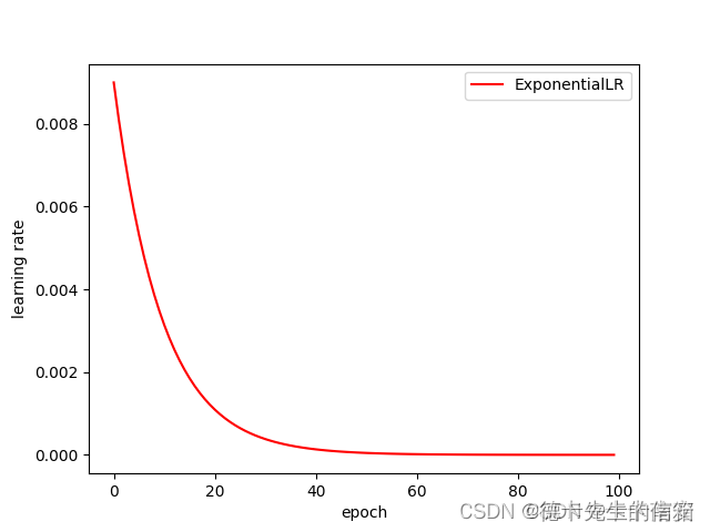
2.4 ExponentialLR(指数衰减)

每个epoch中lr都乘以gamma
torch.optim.lr_scheduler.ExponentialLR(optimizer, gamma, last_epoch=-1)
optimizer：封装的优化器
gamma ：学习率衰减的乘数因子
last_epoch：最后一个迭代epoch的索引，默认为-1
# 其他代码与LambdaLR中相同
scheduler = lr_scheduler.ExponentialLR(optimizer, gamma=0.9)

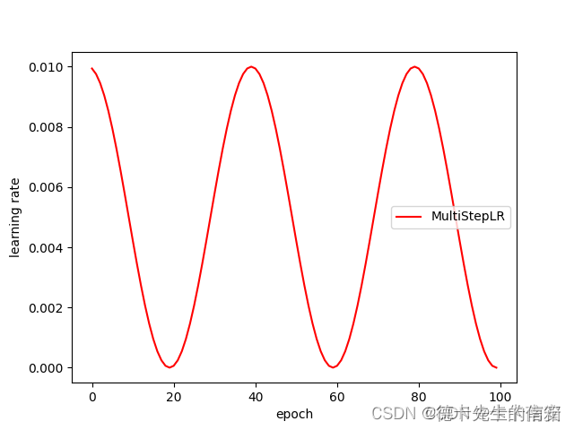
2.5 CosineAnnealingLR(余弦退火衰减)

使得学习率按照余弦函数周期变化

torch.optim.lr_scheduler.CosineAnnealingLR(optimizer, T_max, eta_min=0, last_epoch=-1)

optimizer：封装的优化器
T_max：表示余弦函数周期
eta_min：表示学习率的最小值，默认它是0表示学习率至少为正值。
last_epoch：最后一个迭代epoch的索引，默认为-1

确定一个余弦函数需要知道最值和周期，其中周期就是T_max，最值是初始学习率。
#其他代码与LambdaLR中相同
scheduler = lr_scheduler.CosineAnnealingLR(optimizer, T_max = 20)

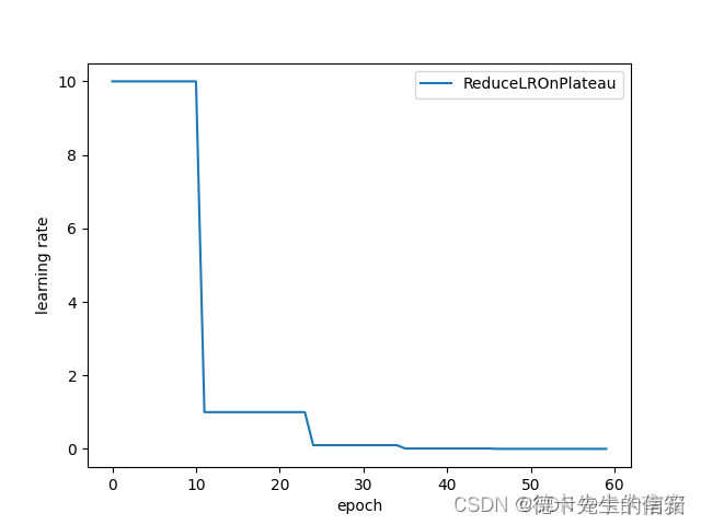
2.6 ReduceLROnPlateau(动态衰减学习率)

基于一些验证测量对学习率进行动态的下降当评价指标停止改进时，降低学习率。一旦学习停滞不前，模型通常会从将学习率降低2-10倍中获益。这个调度器读取一个度量量，如果在“patience”迭代内没有看到改进，那么学习率就会降低。
比如第一个loss为0.71542，一直向后的patient=10的10个epoch中都没有loss小于它，所以根据mode=‘min’，lr = lr*factor=lr * 0.1,所以lr从10变为了1.0

torch.optim.lr_scheduler.ReduceLROnPlateau(optimizer, mode='min', factor=0.1, patience=10, verbose=False, threshold=0.0001, threshold_mode='rel', cooldown=0, min_lr=0, eps=1e-08)

optimizer (Optimizer)：封装的优化器
mode (str)：min, max两个模式中一个。在min模式下，当监测的数量停止下降时，lr会减少;在max模式下，当监视的数量停止增加时，它将减少。默认值:“分钟”。
factor (float)：学习率衰减的乘数因子。new_lr = lr * factor. Default: 0.1.
patience (int)：没有改善的迭代epoch数量，这之后学习率会降低。例如，如果patience = 2，那么我们将忽略前2个没有改善的epoch，如果loss仍然没有改善，
    		那么我们只会在第3个epoch之后降低LR。Default:10。
verbose (bool)：如果为真，则为每次更新打印一条消息到stdout. Default: False.
threshold (float)：阈值，为衡量新的最优值，只关注显著变化. Default: 1e-4.
threshold_mode (str)：rel, abs两个模式中一个. 在rel模式的“max”模式下的计算公式为dynamic_threshold = best * (1 + threshold)，或在“min”模式下的公式为best * (1 - threshold)。
    		在abs模式下的“max”模式下的计算公式为dynamic_threshold = best + threshold，在“min”模式下的公式为的best - threshold. Default: ‘rel’.
cooldown (int)：触发一次条件后，等待一定epoch再进行检测，避免lr下降过速. Default: 0.
min_lr (float or list)：标量或标量列表。所有参数组或每组的学习率的下界. Default: 0.
eps (float)：作用于lr的最小衰减。如果新旧lr之间的差异小于eps，则忽略更新. Default: 1e-8.

2.7 其他