Normalization-归一化层-CSDN博客

本文链接：https://blog.csdn.net/weixin_43687366/article/details/108572992

1、为什么使用normalization?

主要还是为了克服神经网络难以训练的弊端！internal covariate shift:数据尺度/分布异常，导致训练困难！

具体详解请移步：知乎关于normalization的介绍讲解的很详细，我这里也不多赘述了！

2、Pytorch中常见的Normalization有哪些？

Layer Normalization(LN)：BN不适用于变长的网络，如RNN
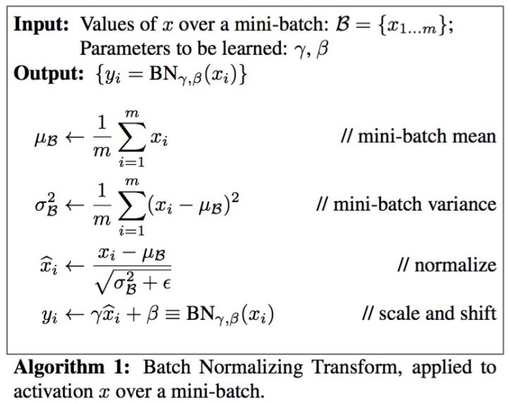
Batch Normalization(BN)：
Instance Normalization(IN)：逐通道计算均值和方差
Group Normalization(GN)：小batch样本中，BN估计的值不准；数据不够，通道来凑；

它们的相同点就是计算公式都一样，只是其中的均值和方差的计算方式不一样；

下面就一个个来看一下原理和代码实现！

2.1、Layer Normalization(LN)

注意事项：gamma和beta为逐元素的；每一层元素都有属于自己的不同的gamma和beta；

LayerNorm(normalized_shape, eps=1e-05, elementwise_affine=True)

$y = \frac{x - \mathrm{E}[x]}{ \sqrt{\mathrm{Var}[x] + \epsilon}} * \gamma + \beta$

其中gamma和beta都是可学习的参数；`affine`选项对每个整个通道/平面应用标量缩放和偏差，“层归一化”使用：参数`elementwise_affine`应用每个元素的缩放和偏差。一般默认是True。参数初始化为1（用于权重）和0（用于偏差）。

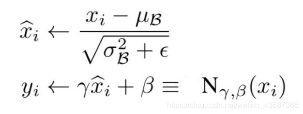
其中的gamma和beta都是逐元素的，逐层计算均值和方差；

上述公式中的均值E[x]和方差Var[x]通过下面方式计算；

normalized_shape（int或list或torch.Size）：来自预期大小的输入的输入形状；

$[* \times \text{normalized\_shape}[0] \times \text{normalized\_shape}[1] \times \ldots \times \text{normalized\_shape}[-1]]$

如果使用单个整数，则将其视为一个单例列表，并且此模块将在最后一个预期为该特定大小的维度上进行规范化。

eps：为分数值增加的分母值。默认值：1e-5

代码实现：

import torch
import numpy as np
import torch.nn as nn
import random

# 设置随机种子
def set_seed(seed=1):
    random.seed(seed)
    np.random.seed(seed)
    torch.manual_seed(seed)
    torch.cuda.manual_seed(seed)

set_seed(1)

# Layer Normalization
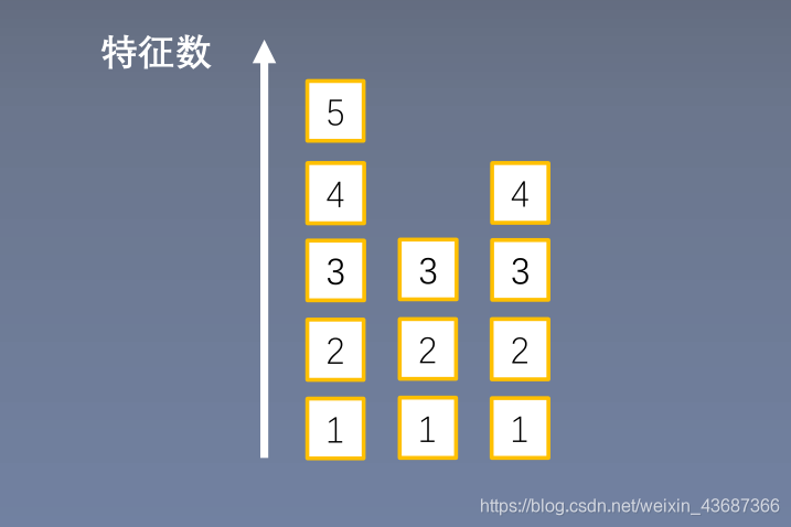
batch_size = 8
num_features = 6
features_shape = (3,4)

feature_map = torch.ones(features_shape)
# [6,3,4]
feature_maps = torch.stack([feature_map*(i+1) for i in range(num_features)],dim=0)
# [8,6,3,4]
feature_maps_bs = torch.stack([feature_maps for i in range(batch_size)],dim=0)

# 从dim=1开始，进行layerNormalization: [B*C*H*W]
# ln = nn.LayerNorm(feature_maps_bs.size()[1:],elementwise_affine=True)
# ln = nn.LayerNorm(feature_maps_bs.size()[1:],elementwise_affine=False)
ln = nn.LayerNorm([6,3,4])
output = ln(feature_map_bs)

print("layer normalization")
# 当将elementwise_affine设置为False时，就会出错，因为就没有权重初始化，怎么可能有形状，还是使用默认值True
# print(ln.weight.shape)
print(feature_maps_bs.shape)
print(feature_maps_bs[0,...])
print(output[0,...])

layer normalization
torch.Size([8, 6, 3, 4])
tensor([[[1., 1., 1., 1.],
         [1., 1., 1., 1.],
         [1., 1., 1., 1.]],

        [[2., 2., 2., 2.],
         [2., 2., 2., 2.],
         [2., 2., 2., 2.]],

        [[3., 3., 3., 3.],
         [3., 3., 3., 3.],
         [3., 3., 3., 3.]],

        [[4., 4., 4., 4.],
         [4., 4., 4., 4.],
         [4., 4., 4., 4.]],

        [[5., 5., 5., 5.],
         [5., 5., 5., 5.],
         [5., 5., 5., 5.]],

        [[6., 6., 6., 6.],
         [6., 6., 6., 6.],
         [6., 6., 6., 6.]]])
tensor([[[-1.4638, -1.4638, -1.4638, -1.4638],
         [-1.4638, -1.4638, -1.4638, -1.4638],
         [-1.4638, -1.4638, -1.4638, -1.4638]],

        [[-0.8783, -0.8783, -0.8783, -0.8783],
         [-0.8783, -0.8783, -0.8783, -0.8783],
         [-0.8783, -0.8783, -0.8783, -0.8783]],

        [[-0.2928, -0.2928, -0.2928, -0.2928],
         [-0.2928, -0.2928, -0.2928, -0.2928],
         [-0.2928, -0.2928, -0.2928, -0.2928]],

        [[ 0.2928,  0.2928,  0.2928,  0.2928],
         [ 0.2928,  0.2928,  0.2928,  0.2928],
         [ 0.2928,  0.2928,  0.2928,  0.2928]],

        [[ 0.8783,  0.8783,  0.8783,  0.8783],
         [ 0.8783,  0.8783,  0.8783,  0.8783],
         [ 0.8783,  0.8783,  0.8783,  0.8783]],

        [[ 1.4638,  1.4638,  1.4638,  1.4638],
         [ 1.4638,  1.4638,  1.4638,  1.4638],
         [ 1.4638,  1.4638,  1.4638,  1.4638]]], grad_fn=<SelectBackward>)

2.2、Batch Normalization(BN)

关于BN，pytorch中提供了三个

nn.BatchNorm1d
nn.BatchNorm2d
nn.BatchNorm3d

(1) nn.BatchNorm1d

BatchNorm1d(num_features, eps=1e-05, momentum=0.1, affine=True, track_running_stats=True)

$y = \frac{x - \mathrm{E}[x]}{\sqrt{\mathrm{Var}[x] + \epsilon}} * \gamma + \beta$

$\hat{x}$ 表示估计的统计量， $x_t$ 表示新的观测值；均值和标准差在最小批次的每个维度上进行计算，并且 $\gamma$ 和 $\beta$ 都是可学习的参数向量，大小为输入大小；并且 $\gamma$ 和 $\beta$ 的默认值分别为 1 和 0；

动量：momentum默认值为0.1；更新准则为：

$\hat{x}_\text{new} = (1 - \text{momentum}) \times \hat{x} + \text{momentum} \times x_t$

其中 $\hat{x}$ 是估计值数据， $x_t$ 是新观测值数据；

参数：

num_features：输入大小（N，C，L）中的 C 或者输入大小（N，L）中的 L;

eps：在公式分母上增加的数值以保证数值稳定性，默认为1e-5；

momentum：用于running_mean和running_var的计算，默认为0.1；

affine：布尔值，设置为True时表示这个模块有可学习的仿射参数，默认也是True;

track_running_stats：设置为True时表示会记录运行时的mean和var，当设置为False时就不会记录；默认为True;

# 输入和输出的尺度是一样的
m = nn.BatchNorm1d(2)
m1 = nn.BatchNorm1d(2,affine=False)
input = torch.randn(2,2)
output = m(input)
output1 = m1(input)

print(output,output1)
print(output.shape,output1.shape)

tensor([[ 0.9999, -1.0000],
        [-0.9999,  1.0000]], grad_fn=<NativeBatchNormBackward>) tensor([[ 0.9999, -1.0000],
        [-0.9999,  1.0000]])
torch.Size([2, 2]) torch.Size([2, 2])

(2) nn.BatchNorm2d

BatchNorm2d(num_features, eps=1e-05, momentum=0.1, affine=True, track_running_stats=True)

这里的参数和上述BatchNorm1d的情况是一样的

# 输入和输出的形状是一样的：[N,C,H,W] => [N,C,H,W]
# 因为Batch Normalization是在通道 C维度上计算统计量，因此也称为Spatial Batch Normalization
m = nn.BatchNorm2d(2, affine=False)
input = torch.randn(2,2,3,3)
output = m(input)
print(output)

(3) nn.BatchNorm3d

# [N, C, D, H, W] 输入等于输出
m = nn.BatchNorm3d(100)
input = torch.randn(20,100,35,45,10)
output = m(input)
print(output.shape)

2.3、Instance Normalization(IN)

起因：BN在图像生成中不适用

思路：逐通道计算均值和方差

主要参数：

num_features：一个样本特征数量

eps：分母修正项

momentum：指数加权平均估计当前mean和var

affine：是否需要affine transform

track_running_stats：是训练状态，还是测试状态

m = nn.InstanceNorm2d(2)
input = torch.randn(2,2,3,3)
output = m(input)
print(output.shape)

torch.Size([2, 2, 3, 3])

2.4、Group Normalization(GN)

 GroupNorm(num_groups, num_channels, eps=1e-05, affine=True)

主要参数：

num_groups:分组数

num_channels:通道数（特征数）

eps:分母修正项

affine：是否需要affine transform

input = torch.randn(2,6,10,10)
# 将6通道分为3组
m = nn.GroupNorm(3,6)
# 将6通道分为6组
m1 = nn.GroupNorm(6,6)
# 将6通道分为1组
m2 = nn.GroupNorm(1,6)

output = m(input)
print(output.shape)

总结：总的来说，只要搞懂一个，其他几个参数基本上都是差不多，最大的不同点就是它们计算均值和方差的方式不同；