


Reinforcement Learning Problems
Overview
1)What is Reinforcement Learning?
2)Markov Decision Processes
3)Q-Learning
4)Policy Gradients
1.”Markov Decision Process”
Abstract:
Problems involving an agent interacting with an environment,which provides numeric reward signals.
①:Agent:take actions in its environment,and it can receive rewards for its action.
②:Agent’s goal:learn how to take actions in a way that can maximize its reward.
③:Set up:How can we mathematically formalize the PL problem?
1)Markov Property:
The current state completely characterizes the state of the world.Defined by tuples of projects:(S,A,R,P,γ)
S: set of possible states
A: set of possible actions
R: distribution of reward given (state,action) pair
P: transition probability i.e. distribution over next state given (state,action) pair
γ:discount factor
2)The way Markov Decision Process work
First,time step t=0,environment samples initial state S0~P(S0)
Then,for t=0 until done:
— Agent selects action At
— Environment samples reward Rt~R(.|St,At)
— Environment samples next state St+1~P(,|St,At)
— Agent receives reward Rt and next state St+1
Now,based on this,we can define a policy Π,which is a function from S to A that specifies what action to take in each state.
Objective: find policy Π* that maximizes cumulative discounted reward:Σ(t>0)γ’t *R
Question: How do we handle the randomness(initial state, transition probability…)?
To maximize the expected sum of rewards!
–>
3)Formally:
Π*=argmax E[Σ(t>0)γ’t * Rt|Π] with S0~P(S0), At~Π(.|St), St+1~P(.|St,At)
①:Initial state samples form our state distribution.
②:Actions sampled from our policy,given the state.
③:Next states sampled from our transition probability distributions.
④:Definitions:Value function and Q-Value function
Following a policy(Π*) produces sample trajectories(or paths) for every single episode S0,A0,R0,S1,A1,R1… We’re going to have this trajectory of states,actions,and rewards that we get.
How good is a state?
The value function at state S,is the expected cumulative reward from following the policy from state S:
V’s Π(S)=E[Σ(t>=0)γ’s t*Rt|S0=S,Π]
How good is a state-action pair?
The Q-Value function at state S and action A,is the expected cumulative reward from taking action A in state S and then following the policy:
Q’s Π(S,A)=E[(Σ(t>=0)γ’s t*Rt|S0) | (S0=S,A0=A,Π)]
⑤:Bellman equation

First we have randomness over what state that we’re going to end up in.(So we have this expectation)
Then,the optimal policy Π* is going to take the best action in any state as specified by Q*. Q* will tell us of the maximum future reward that we can get from any of our actions.So we should just take a policy that’s going to lead to best reward.
2.Q-Learning
1)Solving for the optimal policy
First idea:Value Iteration Algorithm
At each step,we’re going to refine our appropiximation of Q* by trying to enforce the Bellman equation.

To solve the problem:
2)Q-Learning
Use a function appropiximator to estimate the action-value function.
Q(S,A;θ)≈Q*(S,A) -->θ:function parameters(like weights)
If a function approximator is a deep neural network–>deep Q-Learning!
How do we solve our optimal policy?

3)Q-Network Architecture

Doing (downsampling,cropping…) pre-processing step to get to our actual input state.
Basically,we take our current state in,and then because of we have this output of an function(or Q-Value for each action) as our output layer,we’re able to do one pass and get all of these values out.
To train the Q-Network:
1)Loss function(from before)
2)Experience Replay:
What’s the advantage of this way to train Q-Network?
Learning from batches of consecutive samples is bad.The reason is taking samples of state,action,rewards that we have are just taking consecutive samples of these and training with these,all of these samples are correlated —> CAUSE INEFFICIENT LEARNING! What’s more,the current Q-Network parameters determine next training samples—> CAUSE BAD FEEDBACK LOOPS!
So,to solve these problems,we use Experience Replay.Here are the benefits:
①:Keep this replay memory table of transitions of state (as state,action,reward,next state).We have transitions,and we’re going to continually update this table with new transitions that we’re getting (as game episodes are played that we’ve learned before), as we’re getting more experience.
②:Now we can train our Q-Network on random,minibatches of transitions from the replay memory.So,instead of using consecutive samples,we’re now going to sample across these transitions that we’ve accumulated random samples of these.
③:Another side benifit:Each of these transitions can also contribute to potentially multiple weight updates.We just sampling from this table and we could sample one multiple times.—>Lead also to GREATER DATA EFFICIENCY!
④:Summarize:putting Q-Learning and Experience Replay together

Here sample random minibatch from transitions is Experience Replay.
3.Policy Gradients
What’s the problem with Q-Learning?
The Q-function can be very complicated! For example,arobot grasping an object has a very high-dimensional state —> hard to learn exact value of every (state,action) pair.
Can we learn a policy directly?

How can we do this?
Gradient ascent on policy parameters!
We’ve learned that given some objective that we have,some parameters we can just use gradient assent in order to continuously improve our parameters.
How can we take action to this?
Use “Reinforce Algorithm”!
We’re going to sample these trajectories of experience (like episodes of game play), using some policy Π of θ.And then for each trajectory,we can commpute a reward for that trajectory.it’s the cumulative reward that we gor from following this trajectoryγ,and then the value of policy Π minus θ,to be just the expected reward of these trajectories that we can get from the following Π-θ.

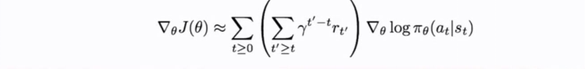
Let’s differentiate this:
①:use Monte Carlo Sampling to estimate
▽θJ(θ)=∫γ(R(γ)▽θlogP(γ;θ))P(γ;θ)dγ = Eγ~P(γ;θ)[R(γ)▽θlog P(γ;θ)]
(P(γ;θ):transition probabilities)
Can we compute those quantities without knowing the transition probabilities? Sure!

If we give one trajectory high reward,then increase the probabilities of all the actions we’ve seen.Otherwise,if the reward is low,then decrease these probabilities,don’t do too much sampling.
②:Intuition–>Gradient Estimator

First,we can do Variance Reduction,this is an important area of research in policy gradients,and in coming up ways in order to improve the estimator and require fewer samples.

Second,we can use Baseline Function,it depends on the state,what’s our guess and what we expect to get from this state,and then our reward or scaling factor that we’re going to use to be pushing up or down our probabilities,can now just be the expected sum of future minus this baseline.So now it’s the relative of how much better or worse is the reward that we got from what we expected.
How do we choose this baseline?
A better baseline:Want to push up the probability of an action from a state,if this action was better than the expected value of what we should get from that state.

Actor-Critic Algorithm
We don’t know Q and V. Can we learn them? Yes!
Using Q-Learning! We can combine Policy Gradinets and Q-Learning by training both an actor(the policy) and a critic(the Q-Function).
The actor decides which action to take, and the critic tells the actor how good its action was and how it should adjust.
Remark: we can define by the advantage function how much an action was better than expected.
AΠ(S,A)=QΠ(S,A)-VΠ(s) (the first A is another meaning,it means advantage function)

Reinforce In Action
-----Recurrent Attention Model(RAM) (also called hard attention model)
Goal: Image Classification
Now you do this by taking a sequences of glimpses around the image,you’re going to look at local regions around the image,basically going to selectively focus on these parts and build up information as you’re looking around,to predict class.
(This is a model that is a capable of extracting information from an image or video by adaptively selecting a sequence of regions or locations and only processing the selected regions at high resolution.)
Instead of processing an entire image or even bounding box at once,at each step,the model selects the next location to attend to based on past information and the demands of the task.Both the number of parameters in our model and the amount of computation it performs can be controlled independently of the size of the input image,which is in contrast to convolutional networks whose computational demands scale linearly with the number of image pixels.
We descirbe an end-to-end optimization procedure uses backpropagation to train the nerual network components and policy gradient to address the non-differentiabilities due to the control problem.
Why we do this?
We consider the attention problem as the sequential decision process of a goal-directed agent interacting with a visual environment.At each point in time,the agent observes the environment only via a bandwidth-limited sensor,i.e. it never senses the environment in full.It may extract information only in a local region or in a narrow frequency band.The agent can,however,actively control how to deplot its sensor resources(e.g. choose the sensor location). The agent can also affect the true state of the environment by excuting actions.Since the environment is only partially observed the agent needs to integrate information over time in order to determine how to act and how to deploy its sensor most effectively. At each step,the agent receives a scalar reward(which depends on the actions the agent has excuted and can be delayed), and the goal of the agent is to maximize the total sum of such rewards.
①:Inspiration from human perception and eye movements.
Look at the complex image–>determine what’s in the image–>look at a low-resolution of it first–>look specifically at parts of the image that will give us clues about what’s in the image.
②:Just look at local regions–>save computational resources–>scalability–>process larger images more efficiently
③:Help with actual classification performance,now you’re able to ignore clutter and irrelevant parts of the image.Means that you can first prune out what are the relevant parts that I actually want to process,using the ConvNet.
What’s the reinforcement learning formulation?
State: Glimpses seen so far
Action: (x,y) coordinates (center of glimpse) of where to look next in image
Reward: 1 at the final timestep if image correctly classified, 0 otherwise
What’s the process?
Glimpsing is a non-differentiable operation–>use reinforcement learning formulation,learn policies how to take these glimpse actions using reinforce.–>Given state of glimpses seen so far, use RNN to model the state and output the next action.
Apply into such as Image Captioning,Visual Question Answering and so on.
4.Summary
Policy Gradients
Very general but suffer from high variance so requires a lot of samples. Challenge:Sample-Effciency
Q-Learning
Does not always work but when it works,usually more sample-efficint. Challenge:Exploration
Guarantees
1)Policy Gradients: Converges to a local minima of J(θ), often good enough!
2)Q-Learning: Zero guarantees since you are approximating Bellman equation with a complicated function approximator.


 596
596


 被折叠的 条评论
为什么被折叠?
被折叠的 条评论
为什么被折叠?
 到【灌水乐园】发言


