【图像处理】基于Zernike矩的亚像素边缘检测理论及MATLAB实现

代码和图片下载

1 边缘检测理论

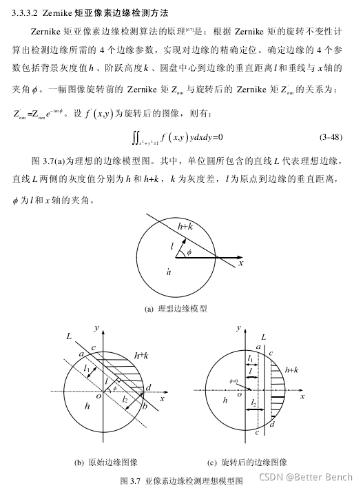
【参考文献】：亚像素边缘检测技术研究_张美静

2 MATLAB实现

function zernike7(I)

I=imread('Pic1_3.bmp');
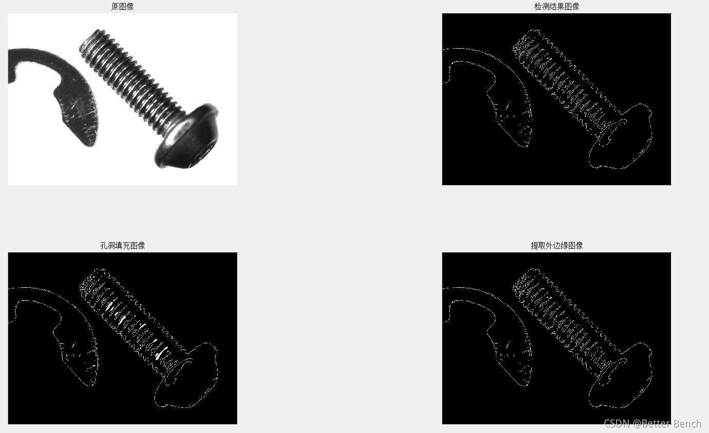
subplot(221)
imshow(I)
title('原图像');
% 7*7Zernike模板
M00=...
[
       0	0.0287	0.0686	0.0807	0.0686	0.0287	0
    0.0287	0.0815	0.0816	0.0816	0.0816	0.0815	0.0287
    0.0686	0.0816	0.0816	0.0816	0.0816	0.0816	0.0686
    0.0807	0.0816	0.0816	0.0816	0.0816	0.0816	0.0807
    0.0686	0.0816	0.0816	0.0816	0.0816	0.0816	0.0686
    0.0287	0.0815	0.0816	0.0816	0.0816	0.0815	0.0287
       0	0.0287	0.0686	0.0807	0.0686	0.0287	0
];
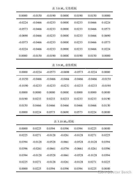
M11R=...
[
       0	-0.015	-0.019	0	0.019	0.015	  0
    -0.0224	-0.0466	-0.0233	0	0.0233	0.0466	0.0224
    -0.0573	-0.0466	-0.0233	0	0.0233	0.0466	0.0573
    -0.069	-0.0466	-0.0233	0	0.0233	0.0466	0.069
    -0.0573	-0.0466	-0.0233	0	0.0233	0.0466	0.0573
    -0.0224	-0.0466	-0.0233	0	0.0233	0.0466	0.0224
       0	-0.015	-0.019	0	0.019	0.015	  0
];
M11I=...
[
       0	-0.0224	-0.0573	-0.069	-0.0573	-0.0224	  0
    -0.015	-0.0466	-0.0466	-0.0466	-0.0466	-0.0466	-0.015
    -0.019	-0.0233	-0.0233	-0.0233	-0.0233	-0.0233	-0.019
       0	   0	   0	   0	   0	   0	  0
    0.019	0.0233	0.0233	0.0233	0.0233	0.0233	0.019
    0.015	0.0466	0.0466	0.0466	0.0466	0.0466	0.015
       0	0.0224	0.0573	0.069	0.0573	0.0224	  0
];
M20=...
[
       0	0.0225	0.0394	0.0396	0.0394	0.0225	0
    0.0225	0.0271	-0.0128	-0.0261	-0.0128	0.0271	0.0225
    0.0394	-0.0128	-0.0528	-0.0661	-0.0528	-0.0128	0.0394
    0.0396	-0.0261	-0.0661	-0.0794	-0.0661	-0.0261	0.0396
    0.0394	-0.0128	-0.0528	-0.0661	-0.0528	-0.0128	0.0394
    0.0225	0.0271	-0.0128	-0.0261	-0.0128	0.0271	0.0225
       0	0.0225	0.0394	0.0396	0.0394	0.0225	0
];


if length(size(I))==3 I=rgb2gray(I); end
I=im2bw(I,0.6);
K=double(I);
[m n]=size(K);
xs=double(zeros(m,n));
ys=double(zeros(m,n));

% 卷积运算
A11I=conv2(M11I,K);
A11R=conv2(M11R,K);
A20=conv2(M20,K);

% 截掉多余部分
A11I=A11I(4:end-3,4:end-3);
A11R=A11R(4:end-3,4:end-3);
A20=A20(4:end-3,4:end-3);

J=zeros(size(K));
boundary=J;
theta=atan2(A11I,A11R);%计算theta

%计算边缘的三个参数
A11C=A11R.*cos(theta)+A11I.*sin(theta);
l=A20./A11C;
k=1.5*A11C./((1-l.^2).^1.5);
e=abs(l)>1/3.5;
k(e)=0;

%边缘判断条件
a=abs(l)<1/sqrt(2)*2/7;
b=abs(k)>max(I(:))/10;
% a,b分别为距离和边缘强度判断结果
J(a&b)=1;
%将图像的最边缘去除
% boundary(2:end-1,2:end-1)=1;
% J(~boundary)=0;
format short
% [x,y]=find(J==1);%边缘的像素级坐标
% O=[x y];
% Z=[x+l(find(J==1)).*cos(theta(find(J==1))) y+l(find(J==1)).*sin(theta(find(J==1)))];%亚像素坐标
% % fprintf('%.4f %.4f\n',Z');

[L,num]=bwlabel(J,8);%对二值图像进行标记
%自动化搜索连通域
s=zeros(1,num);
for i=1:num
   s(i)=size(find(L==i),1);
end
[bwL,label]=sort(s,'descend');
if label(1)<label(2)
    index1=label(1);
    index2=label(2);
else
    index1=label(2);
    index2=label(1);
end

%计算左边探针的最前端坐标
[r1,c1]=find(L==index1);
A1=[r1 c1];
y1=max(A1(:,2));%该连通域中y最大值为针尖处
x1=max(A1(find(A1(:,2)==y1),1));
x1sub=x1+3.5*l(x1,y1)*cos(theta(x1,y1));
y1sub=y1+3.5*l(x1,y1)*sin(theta(x1,y1));

%计算最右边探针的最前端坐标
[r2,c2]=find(L==index2);
A2=[r2 c2];
y2=min(A2(:,2));%该连通域中y最小为连通域
x2=max(A2(find(A2(:,2)==y2),1));
x2sub=x2+3.5*l(x2,y2)*cos(theta(x2,y2));
y2sub=y2+3.5*l(x2,y2)*sin(theta(x2,y2));

% [x1sub y1sub],[x2sub,y2sub]
subplot(222)
imshow(J)
title('检测结果图像');
% figure;
% imcontour(J,1)

% 边界提取
% subplot(122);
% bwimg = bwmorph(J,'remove');
% imshow(bwimg)

subplot(223);
I41=imfill(J,'holes');
imshow(I41)
title('孔洞填充图像');
% 提取最外围边缘
subplot(224);
I4=bwperim(I41);                   
imshow(I4); 
title('提取外边缘图像');
% 去除面积小于150px物体
% subplot(224); 
% I5=bwareaopen(I4,100);    
% imshow(I5);
% title('去除小面积边缘图像');

（1）实验图