R语言两个ROC的比较_不同roc曲线对比采用什么方法-CSDN博客

本文链接：https://blog.csdn.net/weixin_43935907/article/details/123599869

一、概述

ROC是以真阳性率（灵敏度）为纵坐标，以假阳性率（特异度）为纵坐标所绘制的曲线，可以通过不同截断点下的ROC曲线下的面积（AUC），可用于判断该检验方法的诊断价值，正好解决了敏感度和特异度的选择问题。如果AUC小于0.5则表示试验无诊断价值，另外AUC面积越大，表明实验的准确性越高。但是如果两个试验参数的AUC面积都大于0.5，那我们该如何比较这两个ROC指标的诊断能力是否有差别呢？

二、数据集展示

这里就不以科研数据来做展示了，防止泄露个人研究信息，统一采用R语言自带的数据集，接下来就使用pROC自带的数据集aSAH进行演示：

> library(pROC)
Type 'citation("pROC")' for a citation.

载入程辑包：‘pROC’

The following object is masked _by_ ‘.GlobalEnv’:

    aSAH

The following objects are masked from ‘package:stats’:

    cov, smooth, var

Warning message:
程辑包‘pROC’是用R版本4.0.5 来建造的 
> data(aSAH)
> head(aSAH)
   gos6 outcome gender age wfns s100b  ndka
29    5    Good Female  42    1  0.13  3.01
30    5    Good Female  37    1  0.14  8.54
31    5    Good Female  42    1  0.10  8.09
32    5    Good Female  27    1  0.04 10.42
33    1    Poor Female  42    3  0.13 17.40
34    1    Poor   Male  48    2  0.10 12.75

三、两个ROC的比较

1. 比较

> roc_model1 <- roc(outcome~age,data=aSAH) #roc曲线模型1
Setting levels: control = 0, case = 1
Setting direction: controls < cases
> roc_model2 <- roc(outcome~s100b,data=aSAH) #roc曲线模型2
Setting levels: control = 0, case = 1
Setting levels: control = 0, case = 1
Setting direction: controls < cases
> roc.test(roc_model1,roc_model2)

        DeLong's test for two correlated ROC curves

data:  roc_model1 and roc_model2
Z = -1.7604, p-value = 0.07835
alternative hypothesis: true difference in AUC is not equal to 0
sample estimates:
AUC of roc1 AUC of roc2 
  0.6150068   0.7313686

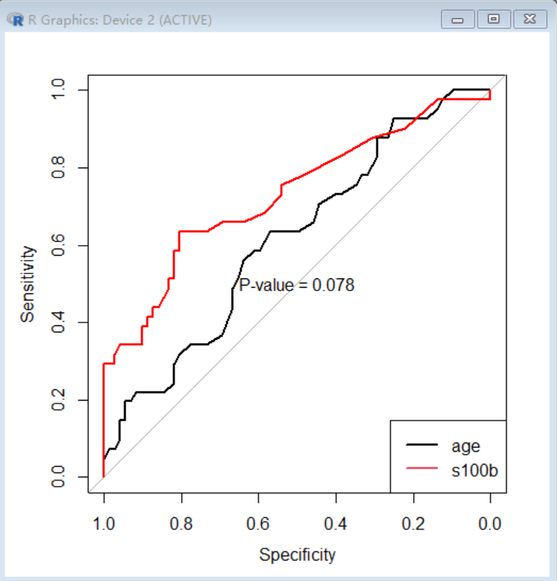
2. 画图

> plot(roc_model1) # 画出roc_model1的roc曲线
> lines(roc_model2,col="red") # 将roc_model2的roc曲线追加到model1的图中
> test <- roc.test(roc_model1,roc_model2) # 获取比较结果并赋值给test
> text(0.5,0.5,labels = paste("P-value =",round(test$p.value,3))) # 将比较结果p值展示在图中
> legend("bottomright",legend=c("age","s100b"),col=c(1,2),lwd = 2) # 画出legend框
>