二手车价格预测-- task3 特征工程

数据预处理和特征选择是数据挖掘与机器学习中关注的重要问题，坊间常说：数据和特征决定了机器学习的上限，而模型和算法只是逼近这个上限而已。特征工程就是将原始数据转化为有用的特征，更好的表示预测模型处理的实际问题，提升对于未知数据的预测准确性。

3.1特征工程

常见的特征工程包括:

1. 异常值的处理:

• 通过箱线图(或3-Sigma)分析删除异常值;
• BOX-COX转换(处理有偏分布);
• 长尾截断;

2. 特征归一化/标准化:

• 标准化(转换为标准正态分布);
• 归一化(转换到[0,1]区间);
• 针对幂律分布,可以采用公式:Log((1+x)/(1+median));

3. 数据分桶

• 等频分桶;
• 等距分桶;
• Best-KS分桶(类似利用基尼指数进行二分类);
• 卡方分桶;

4. 缺失值处理

• 不处理(针对类似XGBoost等树模型);
• 删除(缺失数据太多);
• 插值补全，包括均值/中位数/众数/建模预测/多重插补/压缩感知补全/矩阵补全等;
• 分箱，缺失值一个箱;

5. 特征构造

• 构造统计量特征，报告计数、求和、比例、标准差等；
• 时间特征，包括相对时间和绝对时间，节假日，双休日等；
• 地理信息，包括分箱，分布编码等方法；
• 非线性变换，包括log/平方/根号等；
• 特征组合，特征交叉；
• 仁者见仁，智者见智。

6. 特征筛选

• 过滤式：先对数据进行特征选择，然后再训练学习器，常见的方法有Relief/方差选择法/相关系数法/卡方检验法/- 互信息法；
• 包裹式：直接把最终将要使用的学习器的性能作为特征子集的评价标准，常见方法有LVM；
• 嵌入式：结合过滤式和包裹式，学习器训练过程中自动选择了特征选择，常见的有lasso回归；

7. 降维

• PCA/LDA/ICA；
• 特征选择也是一种降维。

3.2 具体实现

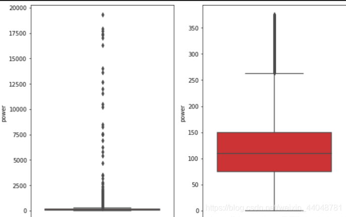
1、删除异常值

借用Datawhale提供的一个函数来处理异常值的代码。

def outliers_proc(data, col_name, scale=3):
    """
    用于清洗异常值，默认用 box_plot（scale=3）进行清洗
    :param data: 接收 pandas 数据格式
    :param col_name: pandas 列名
    :param scale: 尺度
    :return:
    """

    def box_plot_outliers(data_ser, box_scale):
        """
        利用箱线图去除异常值
        :param data_ser: 接收 pandas.Series 数据格式
        :param box_scale: 箱线图尺度，
        :return:
        """
        iqr = box_scale * (data_ser.quantile(0.75) - data_ser.quantile(0.25))
        val_low = data_ser.quantile(0.25) - iqr
        val_up = data_ser.quantile(0.75) + iqr
        rule_low = (data_ser < val_low)
        rule_up = (data_ser > val_up)
        return (rule_low, rule_up), (val_low, val_up)

    data_n = data.copy()
    data_series = data_n[col_name]
    rule, value = box_plot_outliers(data_series, box_scale=scale)
    index = np.arange(data_series.shape[0])[rule[0] | rule[1]]
    print("Delete number is: {}".format(len(index)))
    data_n = data_n.drop(index)
    data_n.reset_index(drop=True, inplace=True)
    print("Now column number is: {}".format(data_n.shape[0]))
    index_low = np.arange(data_series.shape[0])[rule[0]]
    outliers = data_series.iloc[index_low]
    print("Description of data less than the lower bound is:")
    print(pd.Series(outliers).describe())
    index_up = np.arange(data_series.shape[0])[rule[1]]
    outliers = data_series.iloc[index_up]
    print("Description of data larger than the upper bound is:")
    print(pd.Series(outliers).describe())
    
    fig, ax = plt.subplots(1, 2, figsize=(10, 7))
    sns.boxplot(y=data[col_name], data=data, palette="Set1", ax=ax[0])
    sns.boxplot(y=data_n[col_name], data=data_n, palette="Set1", ax=ax[1])
    return data_n

train = outliers_proc(train, 'power', scale=3)

2、特征构造

# 训练集和测试集放在一起，方便构造特征
train['train']=1
test['train']=0
data = pd.concat([train, test], ignore_index=True, sort=False)
# 使用时间：data['creatDate'] - data['regDate']，反应汽车使用时间，一般来说价格与使用时间成反比
# 不过要注意，数据里有时间出错的格式，所以我们需要 errors='coerce'
data['used_time'] = (pd.to_datetime(data['creatDate'], format='%Y%m%d', errors='coerce') - 
                            pd.to_datetime(data['regDate'], format='%Y%m%d', errors='coerce')).dt.days
#查看空数据的数量
data['used_time'].isnull().sum()
# 从邮编中提取城市信息，因为是德国的数据，所以参考德国的邮编，相当于加入了先验知识
data['city'] = data['regionCode'].apply(lambda x : str(x)[:-3])
# 计算某品牌的销售统计量，同学们还可以计算其他特征的统计量
# 这里要以 train 的数据计算统计量
train_gb = train.groupby("brand")
all_info = {}
for kind, kind_data in train_gb:
    info = {}
    kind_data = kind_data[kind_data['price'] > 0]
    info['brand_amount'] = len(kind_data)
    info['brand_price_max'] = kind_data.price.max()
    info['brand_price_median'] = kind_data.price.median()
    info['brand_price_min'] = kind_data.price.min()
    info['brand_price_sum'] = kind_data.price.sum()
    info['brand_price_std'] = kind_data.price.std()
    info['brand_price_average'] = round(kind_data.price.sum() / (len(kind_data) + 1), 2)
    all_info[kind] = info
brand_fe = pd.DataFrame(all_info).T.reset_index().rename(columns={"index": "brand"})
data = data.merge(brand_fe, how='left', on='brand')
数据分桶
bin = [i*10 for i in range(31)]
data['power_bin'] = pd.cut(data['power'], bin, labels=False)
data[['power_bin', 'power']].head()

# 利用好了，就可以删掉原始数据了
data = data.drop(['creatDate', 'regDate', 'regionCode'], axis=1)
# 目前的数据其实已经可以给树模型使用了，所以我们导出一下
data.to_csv('data_for_tree.csv', index=0)

# 我们可以再构造一份特征给 LR NN 之类的模型用
# 之所以分开构造是因为，不同模型对数据集的要求不同
# 我们看下数据分布：
data['power'].plot.hist()

#用肠胃分布截断来代替
train['power'].plot.hist()
data['kilometer'].plot.hist()

data['kilometer'] = ((data['kilometer'] - np.min(data['kilometer'])) / 
                        (np.max(data['kilometer']) - np.min(data['kilometer'])))
data['kilometer'].plot.hist()

# 除此之外 还有我们刚刚构造的统计量特征：
# 'brand_amount', 'brand_price_average', 'brand_price_max',
# 'brand_price_median', 'brand_price_min', 'brand_price_std',
# 'brand_price_sum'
# 这里不再一一举例分析了，直接做变换，
def max_min(x):
    return (x - np.min(x)) / (np.max(x) - np.min(x))

data['brand_amount'] = ((data['brand_amount'] - np.min(data['brand_amount'])) / 
                        (np.max(data['brand_amount']) - np.min(data['brand_amount'])))
data['brand_price_average'] = ((data['brand_price_average'] - np.min(data['brand_price_average'])) / 
                               (np.max(data['brand_price_average']) - np.min(data['brand_price_average'])))
data['brand_price_max'] = ((data['brand_price_max'] - np.min(data['brand_price_max'])) / 
                           (np.max(data['brand_price_max']) - np.min(data['brand_price_max'])))
data['brand_price_median'] = ((data['brand_price_median'] - np.min(data['brand_price_median'])) /
                              (np.max(data['brand_price_median']) - np.min(data['brand_price_median'])))
data['brand_price_min'] = ((data['brand_price_min'] - np.min(data['brand_price_min'])) / 
                           (np.max(data['brand_price_min']) - np.min(data['brand_price_min'])))
data['brand_price_std'] = ((data['brand_price_std'] - np.min(data['brand_price_std'])) / 
                           (np.max(data['brand_price_std']) - np.min(data['brand_price_std'])))
data['brand_price_sum'] = ((data['brand_price_sum'] - np.min(data['brand_price_sum'])) / 
                           (np.max(data['brand_price_sum']) - np.min(data['brand_price_sum'])))

# 对类别特征进行 OneEncoder
data = pd.get_dummies(data, columns=['model', 'brand', 'bodyType', 'fuelType',
                                     'gearbox', 'notRepairedDamage', 'power_bin'])

print(data.shape)
data.columns

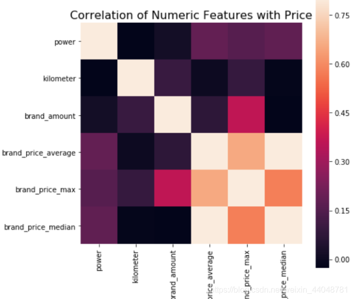
3、特征筛选

# 相关性分析
print(data['power'].corr(data['price'], method='spearman'))
print(data['kilometer'].corr(data['price'], method='spearman'))
print(data['brand_amount'].corr(data['price'], method='spearman'))
print(data['brand_price_average'].corr(data['price'], method='spearman'))
print(data['brand_price_max'].corr(data['price'], method='spearman'))
print(data['brand_price_median'].corr(data['price'], method='spearman'))

# 当然也可以直接看图
data_numeric = data[['power', 'kilometer', 'brand_amount', 'brand_price_average', 
                     'brand_price_max', 'brand_price_median']]
correlation = data_numeric.corr()

f , ax = plt.subplots(figsize = (7, 7))
plt.title('Correlation of Numeric Features with Price',y=1,size=16)
sns.heatmap(correlation,square = True,  vmax=0.8)

总结

因时间安排的比较急，所以匆匆模拟完结果，大概看了一些经典的处理方式与特征工程的一般流程，但是很多细节性的原理不是很理解，需要以后细细看。