简易理解用牛顿法求解方程的根与函数的最值问题（附python demo ）

简易理解用牛顿法求解方程的根与函数的最值问题（附python demo ）

---

1. 先理解基本数学知识

牛顿法用泰勒公式展开是很好理解的。
1.泰勒公式
这里先说明一下，牛顿法和泰勒公式
一阶展开 ：

二阶展开：

2. 牛顿法求根问题

我们知道一个求解简单方程时候，可以通过它的线性变换，最终得到一个解。但是对于一个复杂的根 比如说 求解一个无理数解的时候 。我们是没办法直接算出的解，这时候就需要做一个近似的解代替，这里的近似指的是在误差范围内的近似解。
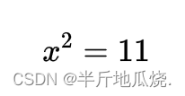
举个例子：求解

这时候就可以用牛顿法做迭代近似才能解出来。

推导过程

• 因为求解一个方程的根，所以方程的左边可以为 0 。 x0 表示初始化的解，x 表示方程的迭代方向解。那么用牛顿法来迭代，
• 肯定是 x = g(x0） 是关于一个x0 的函数迭代更新。我们接下来看这个函数是如果迭代的。

因为是近似解，那么很容易得到：

这就是牛顿法求根问题的更新步骤。牛顿确实牛！
依照这一原理，用牛顿法求根的 步骤为：
因此牛顿法求解方程的根Python伪代码过程为：

1.依照方程定义函数，并求出一阶导数f `(x)
2.初始化 误差 为1 ， 初始化起始值x0;
3.While （误差 >= 10e-5）:
     计算下一个更新自变量x , x_n+1 = x - f(x)/f `(x)
     计算误差f(x_n+1)
     更新 x = x_n+1

得到x 为最终的误差范围内的根。

python代码：

# encoding: utf8
# author: 半斤地瓜烧
# date: 2022年5月24日


import numpy as np
import matplotlib.pyplot as plt


def fun1(x):
    return (x ** 5) - 6


def fun1_de(x):
    return 5 * x ** 4


def fun2(x):
    return np.exp(x) - 4 * np.cos(x)


def fun2_de(x):
    return np.exp(x) + 4 * np.sin(x)


def fun3(x):
    return x ** 2 - np.exp(2 - (x ** 2))


def fun3_de(x):
    return 2 * x + 2 * x * np.exp(2 - (x ** 2))


def fun4(x):
    return 2 * x ** 3 - 9 * x ** 2 + 17 * x + 20


def fun4_de(x):
    return 6 * x ** 2 - 18 * x + 17


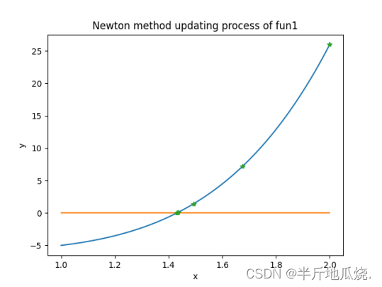
def plot_detail(x_range: list, fun, update: list):
    """
    :param x_range: 题目给出的x 的范围
    :param fun:     原函数
    :param update: 更新的序列
    """
    x = np.linspace(x_range[0], x_range[1], 100)
    fx = fun(x)
    update_arr = np.array(update)
    f_update = fun(update_arr)
    plt.plot(x, fx)
    plt.title("Newton method updating process of {}".format(fun.__name__), )
    plt.xlabel("x")
    plt.ylabel("y")
    plt.plot(x, np.zeros(100))
    plt.plot(update_arr, f_update, "*")
    plt.show()


def newton(fun, fun_de, x_range):
    """
    :param fun: 输入的原函数
    :param fun_de: 原函数的一阶导数
    :param start_x: 牛顿法的输入的起始点
    :return: # 优化参数x,优化后的值fun(x), 优化更新过程的x 列表update_list，优化次数times
    """
    error = 1  # 误差初始化为1 ，只需要大于10e-5即可,在while 中会更新
    x = x_range[1]
    times = 0  # 迭代次数
    update_list = [x]  # x 的更新记录信息

    while error >= 10e-5:  # 当这个误差小于 10e-5 跳出循环 ，x 为最终的优化结果
        x_1 = x - (fun(x) / fun_de(x))  # 牛顿法 更新 x_n+1 = x - f(x)/f`(x)
        update_list.append(x_1)
        error = abs(fun(x_1))  # 计算当前值与跟的 0 的 差距
        x = x_1
        times += 1

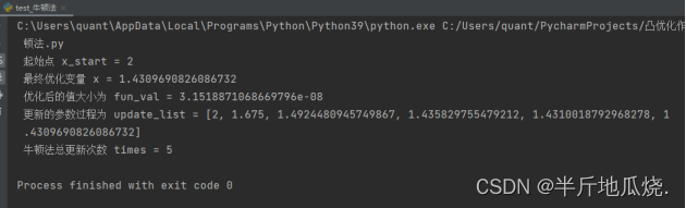
    print(" 起始点 x_start = {} \n 最终优化变量 x = {} \n 优化后的值大小为 fun_val = {} \n "
          "更新的参数过程为 update_list = {} \n 牛顿法总更新次数 times = {}".format(
        x_range[1], x, fun(x),
        update_list,
        times))
    plot_detail(x_range, fun, update_list)


# return x, fun(x), update_list, times  # 优化参数x,优化后的值fun(x), 优化更新过程的x 列表update_list，优化次数times


if __name__ == '__main__':
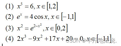
    fun_xrange = [[1, 2], [-1, 1], [0, 2], [-1, 1]]  # 这个列表表示 函数自变量x 的范围
    newton(fun4, fun4_de, fun_xrange[3])

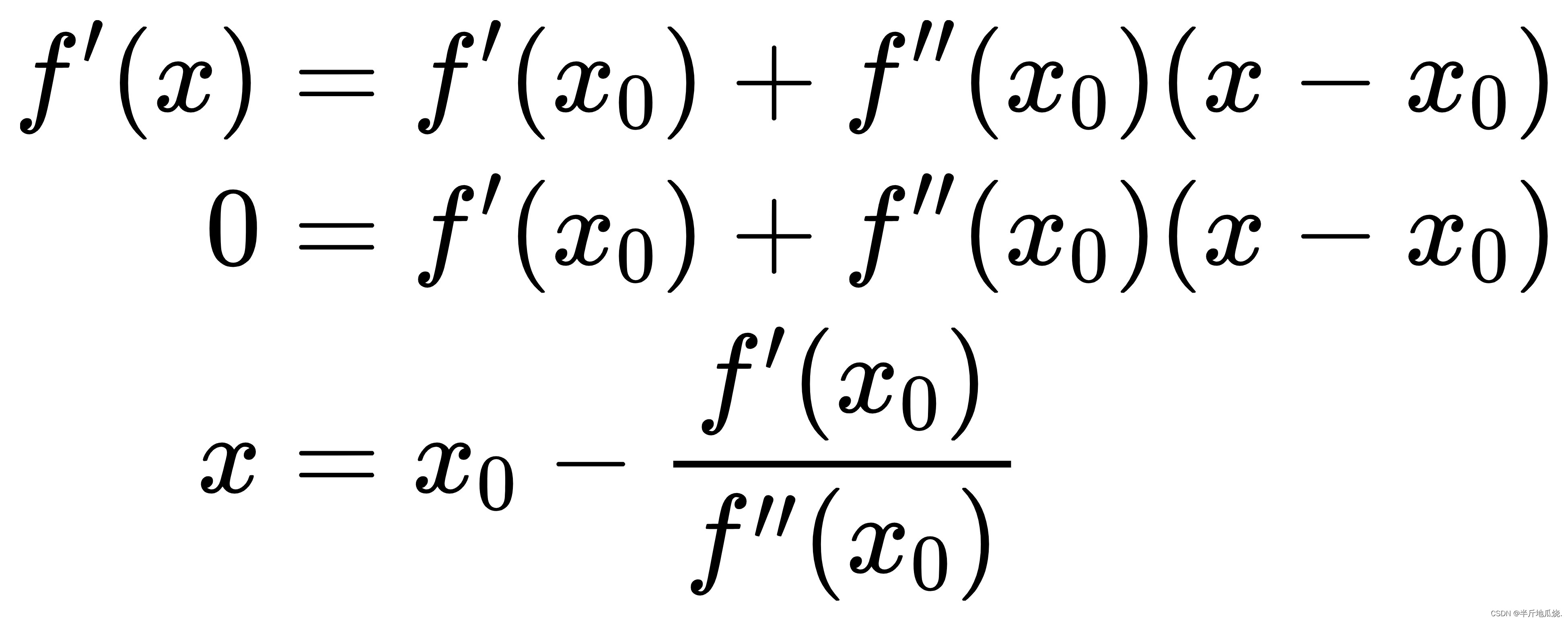
3. 牛顿法求最值问题

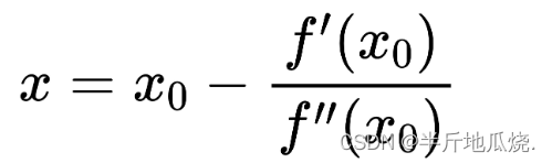
原理，既然求的是最值/极值，那个肯定是一阶导数为0， 在任意函数做泰勒展开之后，求一阶导数，并且令一阶导数为0，即可得出迭代的公式，推导如下：

• 先看一下这个二阶泰勒展开：
  
• 然后上面等式对x求导：

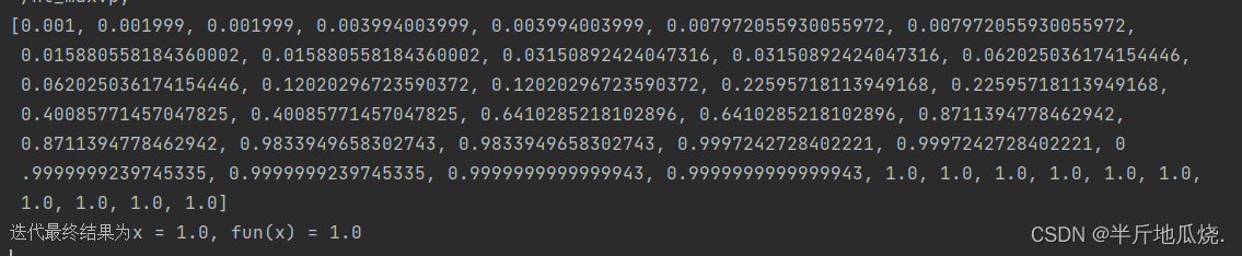
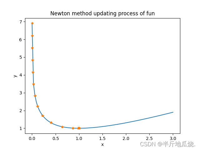
例子：求解 f(x) = x-ln(x) 的最值，看代码与注释：

import numpy as np
import matplotlib.pyplot as plt


def fun(x):
    return x - np.log(x)


def fun_de1(x):
    return 1 - (1 / x)


def fun_de2(x):
    return 1 / (x ** 2)


def newton(fun, fun_de1, fun_de2, start):
    """
    :param fun: 原函数
    :param fun_de1: 一阶导数
    :param fun_de2: 二阶导数
    :param start: 起始点，注意要合法，不能出现分母为0 的情况
    :return: 更新迭代的 x, 以及在误差范围内的最值/极值（除非这个函数是凸函数，这个可以依照函数的二阶条件判断，也就是海森矩阵半正定即可）
    """
    update_list = [start]
    x = start  # 初始化x\

    for i in range(20):
        x_1 = x - (fun_de1(x) / fun_de2(x))  # 牛顿法 更新 x_n+1 = x - f(x)/f`(x)
        update_list.append(x_1)
        error = abs(fun(x_1))  # 计算当前值与跟的 0 的 差距
        x = x_1
        update_list.append(x)
    print("迭代最终结果为x = {}, fun(x) = {}".format(x, fun(x)))

    x = np.linspace(0.001, 3, 100)
    y = fun(x)
    plt.plot(x, y)
    plt.title("Newton method updating process of {}".format(fun.__name__), )
    plt.xlabel("x")
    plt.ylabel("y")
    update_arr = np.array(update_list)
    update_y = fun(update_arr)
    plt.plot(update_arr, update_y, "*")
    plt.show()


if __name__ == '__main__':
    newton(fun, fun_de1, fun_de2, 0.001)

---

以上说的牛顿法求解问题都是很简单的一元函数，但是实际上的参数往往是多元的。这时候只需要求的一阶导数变为 一阶偏导数，二阶偏导数就是Hessian 矩阵，海塞矩阵。详细看《统计学习方法》附录B。

牛顿法的缺点

：

我们看这个迭代公式，首先分母不能为0，也就是海塞矩阵要正定，其二，分母为二阶导，多元时为海塞矩阵 ，因为表示为（分母分之一），也就是需要对海塞矩阵做一个逆运算，这里很复杂的计算步骤。因此基于这个思路，迭代时用一种近似正定矩阵代替了海塞矩阵的逆矩阵/海塞矩阵迭代更新，这种方法就是拟牛顿法。