


逻辑综合
什么是逻辑综合
逻辑综合,是将较高层次的描述自动地转换到较低抽象层次描述的一种方法。这里是指将RTL级的描述转换为门级网表的过程。
逻辑综合要求的输入除RTL描述的程序模块或者原理图文件或波形文件外,还需要另外两个输入文件,第一个输入就是综合工具支持的工艺库(如TTL工艺库,MOS工艺库,CMOS工艺库),这些工艺库中包含一些标准的单元。在综合时,综合工具会将RTL级代码描述的设计用工艺库中的标准单元转化为逻辑电路。另一种输入是约束条件,用于决定综合过程中的逻辑优化方法。约束条件中一般包含时间,面积,速度,功耗,负载要求和优化方法等,甚至还包含综合时需要注意的设计规则。
逻辑综合输出的结果是:门级网表。
逻辑综合步骤:
第一步 (compile):
将RTL描述转换成为未优化的门级布尔描述(如与门,或门,触发器,锁存器等)。该过程不受用户控制,最终转换结果是一种中间结果,格式随不同综合工具而异,对用户不透明,将RTL描述中的IF,CASE,LOOP语句及条件信号代入和选择信号代入语句等转换成中间的布尔表达式。
第二步 (logic optimization):
布尔优化过程,是将一个非优化的布尔描述转化成一个优化的布尔描述的过程。主要是采用某种优化方法,如资源分配、公共子表达式、代码移位、公因子提取、交换律和结合律的运用、死代码消除及常量合并等都是一些基本的优化方法,这一步也称为工艺无关的综合。

第三步 (technology mapping):
门级映射过程,取出经优化的布尔描述,并利用从工艺库中得到的逻辑和定时上的信息去生成门级网表,确保得到的门级网表能达到设计的性能和面积要求。这一步也称为工艺相关的综合(工艺映射),流程图如图。
我们最终将根据优化的布尔描述,工艺库和用户提出的约束条件,将输出一个优化的网表,该网表的结果是以工艺库单元为基础而建成的。
compile
在这里以Verilog开源仿真工具Icarus Verilog为例解释这两个名词的具体含义,这一部分参考自 iVerilog的工作原理,Icarus Verilog是由Stephen Williams开发的Verilog仿真工具,官网http://iverilog.icarus.com,代码开源在https://github.com/steveicarus/iverilog。
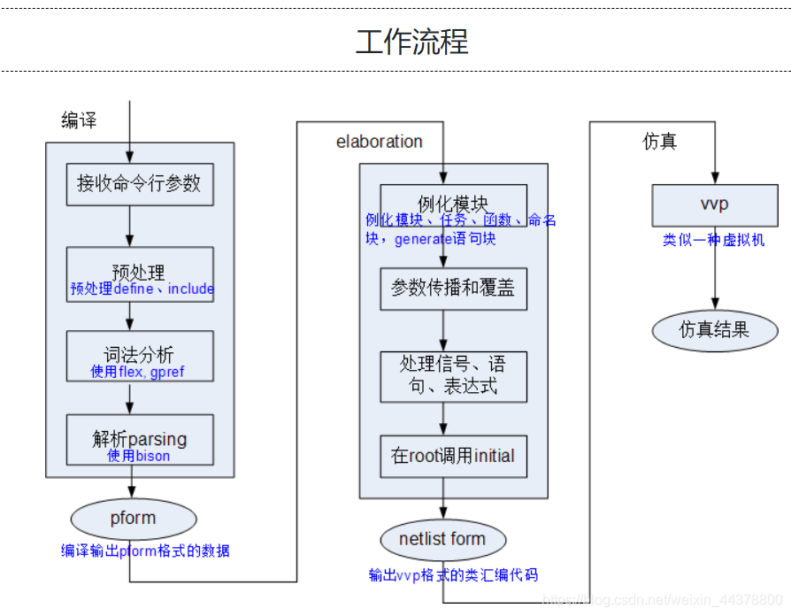
编译就是从接收命令行参数开始,到预处理(verilog宏展开,文件include,条件编译),Verilog语法解析(关键字识别、语法解析),最后转换成内部的数据结构(就是用各种class、结构体,如module、net、scope、generate、statement、expression等)的过程。
简单的讲,就是识别Verilog文件,转成内部的数据库。经过编译后,各个Verilog文件在库里是独立的。
elaboration
elaboration就是把库里的数据,有机的组织成一个树型结构,树的顶端是root,往下是tb或者设计顶层,然后是例化的子模块。如下图:

elaboration的过程中还需要处理parameter的传播、defparam的覆盖,根据generate语句来产生实际的电路等。另外Verilog的系统函数(如 f i n i s h 、 finish、 finish、display、$dumpfile等)也是在这一步进行识别,然后与仿真器预实现的函数库(.so或.a)进行关联。
经过处理后,这个树型结构就可以准确的表达整个设计(包括testbench)。
elaboration还会根据优化选项进行一定的优化,简化树型结构。比如,去除设计层次,用信号命名来表示原层次关系。还可以进行边界优化,合并组合逻辑,合理的优化会很大程度上加速仿真。
术语表
Onset Offset Dont’care(DCset)
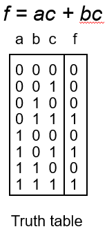
在二级逻辑以及多值逻辑综合优化工具espresso中常会听到关于Onset和Offset的说法,这种说法在电路的PLA逻辑表示中尤为突出,而且在电路的BDD逻辑表示中也有涉及,假定给定一个电路的函数及其真值表如下:
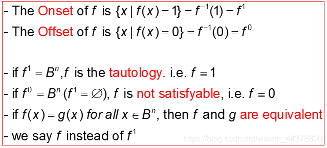
- Onset
函数的Onset是指所有使得函数最终的真值值等于1的最小项的和,例如对于本例的函数而言,Onset=a'bc+ab'c+abc=ac+bc。 - Offset
同理可推导,Offset是指所有使得函数最终的真值值等于0的最小项的和,例如对于本例的函数而言,Offset=a'bc+a'b'c+a'bc'+ab'c'+abc'。 - Dontcare(DCset)
Dontcare在本例中没有得到体现,但是通过上面两例可以推导出一个函数的DCset就是指当函数最终的真值值存在无关项的时候,所有使得函数f结果为无关项x的最小项的和。
Boolean space(B^n)
一个电路函数所有取值的可能性,共有2^n种可能性。
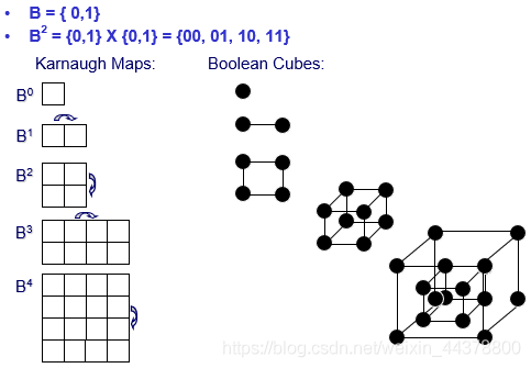
所以对于一个具有n变量的电路逻辑函数,共具有2^n个节点,同时具有2^(2^n)个不同的函数。
TFI TFO logic network
- logic network
Logic networks are directed acyclic graphs (DAGs) composed of logic gates and realizing Boolean functions, which are functions defined over the Boolean space B = { 0 , 1 } , taking primary inputs as inputs and presenting the function outputs at the primary outputs. In this paper, we work with and-inverter graphs (AIGs), but this framework can also be applied to other types of logic networks.
- TFI TFO
该节点所有的扇入(出)节点,一次递归到pi或者po。
A gate in a logic network usually computes a simple function of its fan-ins, and passes the resulting value to all of its fanouts. In the case of AIGs, a gate is always an AND gate, and the inverters are represented by complemented wires with no cost (that is, they do not add to the circuit size). We also refer to a gate as a node. The transitive fan-in (TFI) or the transitive fan-out (TFO) of a node n is a set of nodes such that there is a path between n and these nodes in the direction of fan-in or fan-out, respectively.
literal Cubes List of cubes
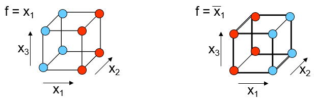
literal通常会翻译为文字,一个文字是指一个变量x或者其反变量x',例如文字x代表逻辑函数f,则f={x|x=1},文字x'代表逻辑函数g,则g={x'|x'=0},如下。
Cube是电路逻辑函数的一种表示方式,放在这里作为一种常用术语以作了解。cube是指一系列文字函数的和(文字数的结合),防止翻译有误,附上英文引用:
A cube is defined as the AND of a set of literals functions (‘conjunction’ of literals).
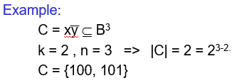
假设对于一个函数C=x1'x2x3',则它用cube表示如下:

同时有以下几点需要注意:
- 如果
C属于函数f且C是一个cube,那么C是函数f的一个蕴涵项。 - 如果
C属于布尔空间B^n且C有k个文字数,那么|C|包含2^(n-k)个顶点。
- 一个具有
n个变量的蕴涵项是一个最小项。
List of cubes说白了就是一系列cubes的集合 (sum of cubes),等价于积之和 (sum of products, SOP),下文中将会有介绍,这里不再做赘述。
DAG FI != PI FO != PO CONE support MFFC
详见本节后附图示例!!!
-
DAG
一个电路可以被表示为一个有向无环图 (Directed Acyclic Graph)C(G,N),其中G代表具体的逻辑门,而N表示连接这些逻辑门的有向边,对于每一个门G都被赋予了一个具体的布尔逻辑函数Fg,该门会根据具体的输入计算出输出。 -
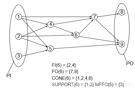
FI
Fanin和primary input的概念不能混淆,前者表示当前该节点所有的前导节点,即该节点的所有扇入–》FI(g)={g'|(g',g) belongs to N},而后者表示该电路所有的原始输入。 -
FO
同上,Fanout和primary output的概念也不能混淆,前者表示当前该节点所有的后导节点,即该节点的所有扇出–》FO(g)={g'|(g',g) belongs to N},而后者表示该电路所有的原始输入。 -
CONE
一个门g的CONE是指该门所有的传导性扇入FI以及它本身。
The CONE(g) of a gate g is the transtive fanin of g and g itself
- SUPPORT
一个门g的SUPPORT是指该门g的所有原始输入PI。
The SUPPORT(g) of a gate g are all inputs inn its cone.
- MFFC
一个节点n或者门g的MFFC是指该门g的扇入CONE的一个子集,该子集中包含了一些节点,这些节点满足的条件是每一条经过这些节点到最终输出PO的路径都需要经过该门g或者该节点n,这样一个FI CONE的子集才能被称作为MFFC。
说白了就是一旦该节点被去除,其部分前导节点不能到达PO的话,那么这些前导节点的集合就是MFFC。
A maximum fanout free cone (MFFC) of a node n is a subset of the fanin cone containing only nodes such that every path from these nodes to the POs passes through n. Informally, if a node is removed, the nodes in its MFFC are also removed.
图示例:对于节点⑥而言,所有的FI CONE为{1,2,4},没有一个扇入满足MFFC的条件,所以该节点不具有MFFC,但是对于节点⑤而言,它的MFFC是 {3}。
Tautology
找到满足条件的解使得函数的值为 0.
Find an assignment to the inputs that evaluate a given vertex to “0”.
SAT
找到一组满足条件的解使得函数的值为 1.
Find an assignment to the inputs that evaluate a given vertex to “1”.
这意味着在对于一个存在反相器的Netlist边进行求解时,SAT和Tautology是等价的。
cover
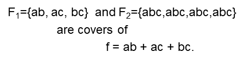
如果函数f是由一系列cube构成的,那么这些cube的集合叫做这个函数f的cover,示例如下。
A set of cubes that represents f is called a cover of f.
cont’d…
Experienced optimization guide from papers.
- Scalable Logic Synthesis using a Simple Circuit Structure, Sec 2.4, Alan, 2006
A tree-like(non-reconvergent) structure does not lead to any don’t-cares in the local space of the node,don’t care may not get better qor for this kind of structure.
1.常用函数逻辑表示
1.1逻辑函数的最小项
根据逻辑函数的概念,一个函数的表达式不是惟一的,例如:
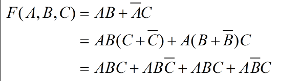
在最后一个函数的表达式中。我们可以看到:
- 每个乘积项都包含了全部输入变量;
- 每个乘积项中的输入变量可以是原变量或者反变量;
- 同一输入变量的原变量和反变量不会同时出现在同一乘积项中。
这样的乘积项我们称之为最小项。
为什么称它为最小项呢?因为对于n个输入,变量的取值组合有2^n种,在这所有的组合中,只有一种是的乘积项的值取1,其他的组合都使得乘积项取0.
全部由最小项相加构成的与-或表达式称之为最小项表达式,这是与-或的标准表达式,也可以被称为标准积之和式(Sum-of-Product,SOP)。
1.2 SOP表示
由函数的最小项的表达式可以看出,任何一个函数都可以表示为SOP的形式,这个不难理解,表达式如下:
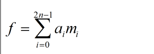
其中mi代表最小项,ai表示该最小项取值1或者0。
1.2.1 SOP变换(RM逻辑)
由前所述,我们知道在一个最小项里面,原变量和反变量不可能同时存在,所以对于任意两个最小项mi和mj(i not equal j)而言,它们“与”的结果都是0,因此“或”运算符可以替换为“异或(Exclusive-OR)”运算符,转换后的表达式如下:
公式一:
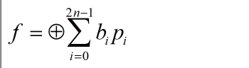
其中bi代表1或者0,pi代表乘积项(i not equal j),更准确的说应该是最小项。
结合前面已经讲到过的,现在我们引入函数不相交的概念,首先我们对于前面的函数SOP表示进行重新的定义:
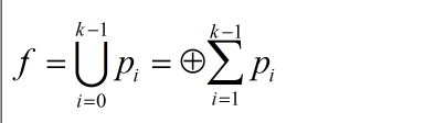
则任意一个n变量函数都可以被表示如下:
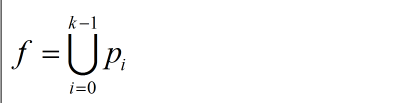
Pi 表示乘积项,k表示乘积项的个数,U表示乘积项之间的逻辑“或”关系,把所有乘积项的集合定义为S,在这里需要注意的是,乘积项与最小项是不同的概念,乘积项包含最小项,对于每一个乘积项Pi,可以改写为最小项的形式:
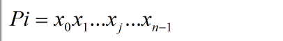
其中x表示变量。
定义1:
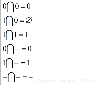
对于两个变量xi,xj,把它们的相交计算记作:
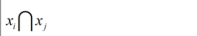
则存在以下表达式,其中“-”表示不确定项:
定义2:
对于两个乘积项,pw和pv(pw、pv属于S且w不等于v),两者的相交运算记作:

若pw和pv存在第i位上(i<=i-1):
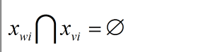
则表示pw和pv不相交,当函数SOP形式的任意两项不相交时,可以将乘积项直接写成以下形式:
公式二:
需要注意的是,这里与公式一的区别在于,公式一是对于最小项可以直接做“异或运算,而这里是在任意两两乘积项不相交的前提下直接做异或运算,也可以称作为传统的Reed-Muller(RM)逻辑,即只包含“与”“异或”运算符。
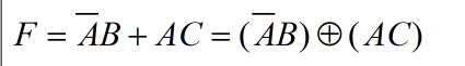
- 示例
在这里举一个例子,例如对于以下表达式,通过定义可以发现两个乘积项是满足不相交定理的,所以可以直接对两个乘积项进行“异或”操作:
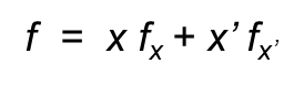
1.2.2 shannon分解
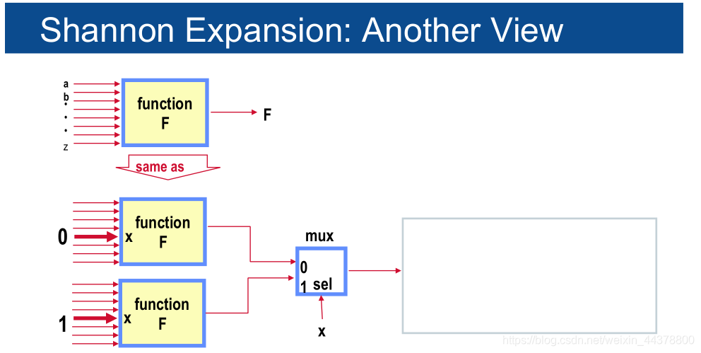
根据前面介绍的SOP的基础知识可以知道,对于任意一个函数,都可以表示为以下的形式(香农展开):

另一种理解的方式如下,可以理解为二选一的MUX,除去变量x或者其反变量后的表达式为MUX的两个输入,而x为选择变量:
- 下面通过一个例子对香农分解进行更好的解释:
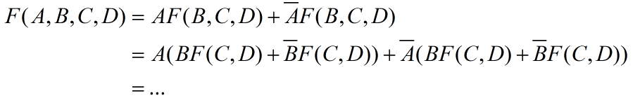
我们会发现到最后一个函数通过香农分解化为了最小项SOP的形式。
1.2.3 shannon cofactor
通过前面的介绍已经知道,任何一个函数都可以通过香农展开写成以下形式:

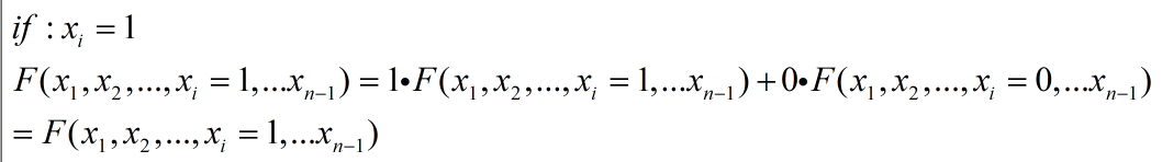
其中对于两个子函数,分别被称为positive-cofactor和negative-cofactor,并且它们等价于表达式F(xi=1)和F(xi=0):

因此,香农展开可以被写作下面这种简单的形式:

此时表达式F(xi=1)是positive cofactor,F(xi=0)是negative cofactor。香农展开也可以通过简单的展开进行证明如下(0同理):
1.2.4 Boolean Derivatives(布尔导数)
TODO
1.3 BDD
1.3.1 BDD
BDD简称为二元决策树,是一种规范的电路(布尔函数、算术函数、代数函数)逻辑表示方式,BDD电路表示主要是基于香农展开:
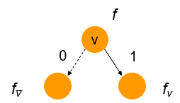
是一种相对于布尔函数而言具有相对紧凑的数据结构,BDD满足以下几个要素:
- 具有一个根节点
root,两个字节点0和1 - 每一个节点都有两个子节点,对应着一个具体的变量
- 是一个香农因子展开树,该项是针对于BDD而言,ROBDD不具备此项
例如对于一个给定电路的逻辑函数如下,最简单(naive way)的BDD表达方式是根据真值表一步一步向下表示如下:
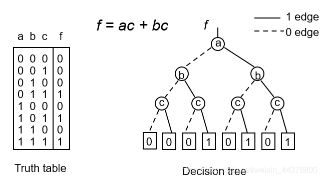
其实BDD所实现函数的功能就是通过指定所有指向1的路径,也就是我们前面所说的Onset,如下示例:
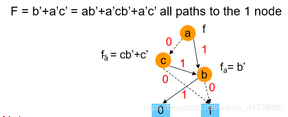
以下是BDD电路逻辑表示的一些优点,为了保证理解的准确性,这里不做翻译,请查看以下引用部分。
- By tracing paths to the 1 node, we get a cover of pair wise disjoint cubes.
- The power of the BDD representation is that it does not explicitly enumerate all paths; rather it represents paths by a graph whose size is measures by its nodes and not paths.
- A DAG can represent an exponential number of paths with a linear number of nodes.
- BDDs can be used to efficiently represent sets
interpret elements of the onset as elements of the set
f is called the characteristic function of that set
1.3.2 OBDD
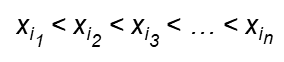
输入变量是有序的排列,即从根节点到最终的0-1的每一条路径的变量顺序一致,示例如下:
1.3.3 ROBDD
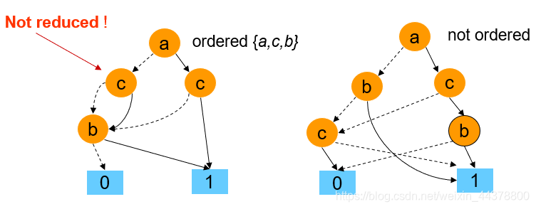
ROBDD全称为reduced ordered BDD,其实从英文全称就可以看出来与BDD相比,ROBDD主要差异体现在reduced和ordered两个方面:
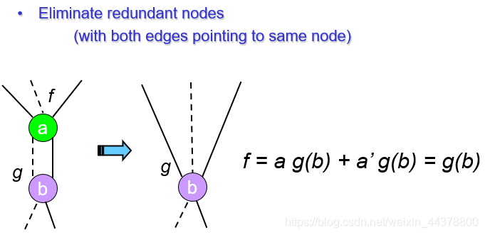
-
Reduced
任何具有两个相同子节点的节点都会被移除,这一过程在一些文献中也被称作为结构性哈希,目的同此 -
Ordered
子节点上的因子变量在所有路劲上始终遵循着同一变量顺序,例如:
接下来给出一个BDD和ROBDD的具体电路表示示意图,可以一目了然的看出二者的差距,当然,具体的BDD逻辑表示会根据用户定义的变量顺序不同而不同。
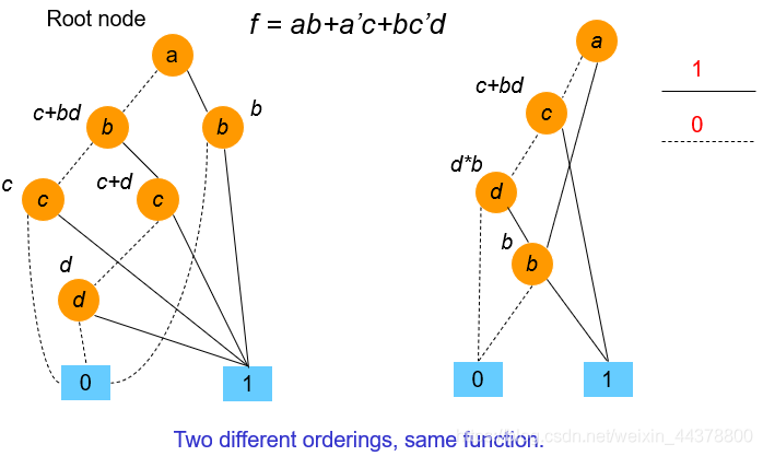
除此之外,ROBDD还要遵循两个减少(reduction)规则: -
Rule1:如果任意节点的两个子节点是相同的,那么该节点将会被删除
-
Rule2: 如果两个图有同构(isomorphic)图,将会用其中一个来替换它们
这两条规则使得每一个节点都可以代表一个不同的逻辑函数,这里针对两条规则举两个示例。
- Rule1
- Rule2

1.3.4 BDD的实现…
1.3.5 BDD的应用场景…
1.4 AIG
-AIG related
A combinational And-Inverter Graph (AIG) is a Boolean network composed of two-input ANDs and inverters. To derive an AIG, the SOPs of the nodes in a logic network are factored, the AND and OR operations of the factored forms are converted into two-input ANDs and inverters using DeMorgan’s rule, and these two-input ANDs are added to the AIG manager in a topological order. The size (area) of an AIG is the number of its nodes; the depth (delay) is the number of nodes on the longest path from the PIs to the POs. The goal of AIG minimization is to reduce both area and delay.
- 结构哈希
Structural hashing of AIGs ensures that all constants are propagated and there is no two-input AND nodes with identical fanins (up to a permutation). Structural hashing is performed on-the-fly by hash-table lookups when AND nodes added to an AIG manager, which helps reduce the AIG size.
- cut
A cut C of a node n is a set of nodes of the network, called leaves of the cut, such that each path from a PI to n passes through at least one leaf. Node n is called the root of cut C. The cut size is the number of its leaves. A trivial cut of a node is the cut composed of the node itself. A cut is K-feasible if the number of leaves in the cut does not exceed K. A cut is dominated if there is another cut of the same node, which is contained, set-theoretically, in the given cut.
- 示例
1.5 MIG…
1.6 XMG…
2.优化算法
2.1 Lazy Man’s Logic Synthesis
paper: Lazy Man’s Logic Synthesis Wenlong, Yang Lingli Wang, Alan Mishchenko
2.1.1 Contributions
一种基于预先计算存储库的电路优化方法。
- A new way of performing logic synthesis. Instead of deriving new circuit structures during runtime of a logic synthesis algorithm, the structure is retrieved from a precomputed library.
- A new way of accumulating circuit structures in a library and hashing them using a semi-canonical form, which trades speed of computation for reduced memory.
- Analysis of the logic synthesis benchmarks to show the number of frequently occurring semi-canonical classes of 12-input functions and how much memory is needed to represent a realistic library of these functions.
- Promising results of delay optimization after FPGA mapping into 4-LUTs and 6-LUTs, obtained using the proposed approach to logic synthesis.
2.1.2 Why proposed ?
总结:保存更多的电路snapshot,期望对于节点进行替换达到面积或者delay最好。
Different tools perform logic synthesis in different ways resulting in different circuit structures. These differences occur because implementations use heuristics and pursue different optimization goals. As a result, there is no “best” circuit structure for a given function. Sometimes even a suboptimal structure may be useful. For example, the result of technology mapping depends on the initial circuit structure [10]. In some cases, a suboptimal circuit before mapping leads to a better result after mapping.
This is why, in many applications, it is desirable to have multiple structural representations of each function. Hence, it is necessary to run different tools and different scripts and produce several structural snapshots of the same design. However, maintaining multiple tools or routinely applying multiple synthesis scripts is expensive and inefficient.
The proposed approach named “lazy man’s logic synthesis” learns from the output of different tools applied to various designs and creates a library of AIG structures. When these structures are available and compactly recorded, there is no need to perform traditional logic synthesis. It is enough to check whether a function is already present in the library. The process of looking up is made fast by hashing functions using an affordable semi-canonical form described in this paper.
2.1.3 Background
- AIG related
Please refer to Section 1.4. - NPN equivalent
Two functions are NPN-equivalent if one of them can be obtained from the other by negation and/or permutation of the inputs and outputs
- positive minterm
A positive minterm is a complete assignment of input variables, which makes the function evaluate to 1.
2.1.4 Algorithm
总结:基于预先计算存储库的优化算法。
LMS is based on collecting, storing, and re-using circuit structures of Boolean functions with 6-12 input variables. Since the total number of completely-specified Boolean functions of N variables is 2(2N), storing all of them is infeasible for N > 4. For larger values of N, only the functions occurring frequently in the benchmarks should be considered. We call such functions practical and give frequency statistics in the experimental results section.
为何只考虑NPN等价类?
However, even the number of practical functions can be very large. To reduce this number and memory needed to store them in a library, they can be broken into equivalence classes using a canonical form. In this case, only representatives of equivalence classes are stored in the library.
- Algorithm 1: Generating semi-canonical form
对于多输入变量的函数,并不计算所有的NPN等价类,只是根据所跑的benchmark计算practical的类,因此称作semi-canonical form,好处是可以节省大量的run time。
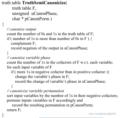
Details: The procedure takes the truth table of a Boolean function and transforms it into a semi- canonical form. This form is the Boolean function of the representative of the equivalence class, to which the given function belongs. First, the output of the function is complimented based on the number of 1s in it. Then, the phase of each variable is decided by the number of the 1s in the negative and positive cofactors. Lastly, the variable ordering is determined by sorting variables using the number of 1s in their cofactors. Variables uCanonPhase and pCanonPerm record the changes in the truth table. They are returned to the calling procedure and later used to determine how to unpermute the subgraphs stored in the library, when this subgraph is used to synthesize a given function.
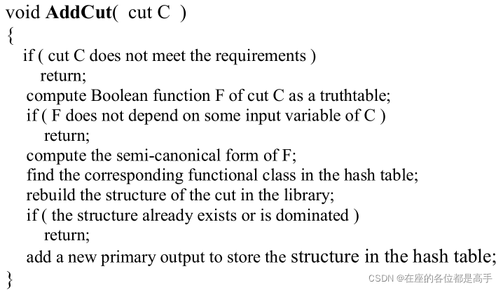
- Algorithm 2: Adding structures to library
预先计算存储的库如何创建
All the optimized structures are stored in the same AIG manager. A library of N-input functions contains also functions with less than N-inputs, but they are remapped to structures which depend on the variables with the smallest variable indexes. Each circuit structure stored in the AIG is identified by a separate primary output.
In this paper, we use the LUT mapper if in ABC as a structural cut browser to generate a fixed number of K-input cuts for each node in benchmark circuits.
Here are the commands for library construction implemented in ABC as part of this work:
- rec_start: Starts the LMS recorder.
- rec_add: Explores cuts of the current network using the cut browser and add useful AIG structures to the library.
- rec_filter: Removes those structures form the library, whose semi-canonical classes appear less frequently than the limit given by
the user.- rec_merge: Merges two previously computed libraries, by combining their circuit structures without the cut browser.
- rec_ps: Prints statistics for the currently loaded library.
- rec_use: Transforms the internal library to the current network in ABC, so it can be written into a file.
- rec_stop: Deletes the current library. Useful before the computation of a new library begins or when it is desirable to free
the memory used by the currently stored library.
- Algorithm 3: Perform LMS on subject graph.
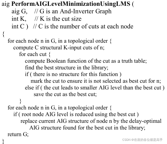
优势:
- SOP balancing uses only one AIG structure derived from an SOP of the function, while LMS has multiple structures to choose from,
including those derived by SOP balancing, if these were harvested
during library computation.- LMS scales to larger functions (up to 12 inputs and more), while SOP balancing works in practice only when the number of variables does not exceed 8.
2.1.5 Result
- 如何创建library
Before the experiment, rec_start is called. After the experiment, rec_use is called, followed by writing the library into a file.
read file; st; rec_add; // add the original AIG structures
• dc2; rec_add; // add structures derived by dc2
• if -K 8; bidec; st; rec_add;
• if -K 8; mfs; st; rec_add;
• if -K 8; bidec; st; rec_add;
• if -g -K 6; st; rec_add;// add structures created by SOP balancing
• if -g -K 6; st; rec_add;
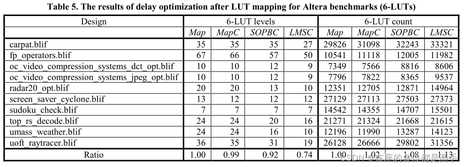
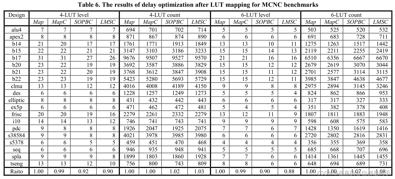
- 实验步骤比较对象
- Map: st; resyn2; if -K 4 or 6
- MapC: st; resyn2; dch -f; if -K 4 or 6
- SOPBC: st; if -gm -K 6; st; resyn2; dch -f; if -K 4 or 6
- LMSC: st; if -ym -K 6; st; resyn2; dch -f; if -K 4 or 6
- 实验结果

2.2 window based resubstitution
2.2.1 Contributions
提出了一种可拓展性更强、效率更高的综合算法。
This paper proposes a resurgence of rewriting and peephole optimization. However, instead of structural matching and rule-based synthesis used in the classical approach, the proposed local transformations rely on efficient modern techniques, such as precomputation, reconvergence analysis, cut enumeration, Boolean matching, exhaustive simulation of small logic cones, and local resource-aware decision procedures based on Boolean satisfiability.
2.2.2 Why proposed ?
有效的将工艺无关和工艺相关的优化分离开,同时也能保持更好的可拓展性、更快的速度、更简洁等,而它能保持住这些特性的原因在于:
- AIG作为同构网络,处理速度较快
- Instead of graph isomorphic and SOP-based optimization, Boolean functions of a group of AIG nodes is computed in terms of various fanin cuts. Several exhaustive and selective cut computations can be used, including a recent development that can efficiently enumerate all cuts up to 12 inputs.
- The Boolean functions of cuts are represented using truth tables. Due to the high speed of bit-parallel manipulation, sub-problems arising in local optimization are often solved, without using SAT or BDDs, by exhaustive simulation, which scales up to 16 inputs.
2.2.3 Background
- 详见术语表以及section 1.4.
Exhaustive simulation
Exhaustive simulation is a practical way of checking equivalence of Boolean function of a node whose size does not exceed 16 inputs. Exhaustive simulation is performed using bitwise simulation of the cone with 2^k different input patterns, where k is the number of leaves. Another way of looking at exhaustive simulation is that it computes the truth-table of the root in terms of the elementary truth-tables set at the leaves.
Windowing
如何根据一个节点创建该节点的window,示例如下:

算法的细节可以通过下图进行深入的理解:

图解:
Figure 2.3.2 shows a 1 × 1 window for node N in a DAG. The nodes labeled I1 , O1 , S, L, and R are in correspondence with the pseudo-code in Figure 2.3.1. The window’s roots (top) and leaves (bottom) are shaded. Note that the nodes labeled by P do not belong to TFI and TFO of N, but represent reconvergent paths in the vicinity of N. The left-most root and right-most root are not in the TFO of N and can be dropped, as explained above
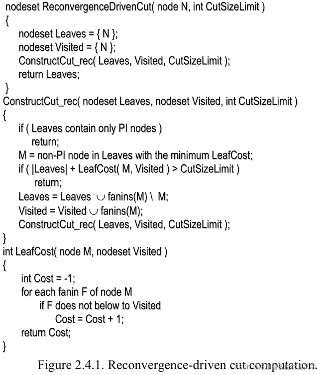
Reconvergence-driven cut computation
当从节点输出开始的路径在到达 PO 之前再次相遇时,就会发生重新收敛.
Reconvergence occurs when the paths starting at the output of a node meet again before reaching the POs. Reconvergence is inevitable due to logic sharing in multi-level logic networks, but excessive reconvergence is often redundant.
- 基于重新收敛的cut计算
Present a simple and efficient cut computation algorithm, which computes a cut close to a given size (if such cut exists) while heuristically maximizing the cut volume and the number of reconvergent paths subsumed in the cut.
2.2.4 Algorithm
Rewriting
- what is rewriting ?
贪心算法在预先计算具有更(最)小面积的库中寻找等价的子电路替换当前的节点,以减少AIG网络的节点数目。
Rewriting is a fast greedy algorithm for minimizing the number of AIG nodes by iteratively selecting AIG subgraphs rooted at a node and replacing them with smaller pre-computed subgraphs, while preserving the functionality of the node.
ABC中的拓展包括以下几点:
• Using 4-input cuts instead of two-level subgraphs.
• Restricting rewriting to preserve the number of logic levels.
• Developing several variations of AIG rewriting that look at
larger subgraphs and/or attempt to reduce the delay.
• Experimental tune-up for logic synthesis applications.
理论上会使用所有的222种NPN类函数,实际上用到的只是其中一部分,原因如下:
For the purposes of AIG rewriting, all 4-feasible cuts of the nodes are found by the fast cut enumeration procedure. For each cut, the Boolean function is computed and its NPN-class is determined by table lookup. Manipulation of 4-variable functions is fast because they are represented using truth tables stored as 16-bit bit-strings. Altogether there are 222 NPN equivalence classes of 4-variable functions, of which only about 100 appear as functions of 4-feasible cuts in any of the available benchmarks, and only about 40 of these have been found experimentally to lead to improvements in rewriting. The unifying characteristic of these 40 remaining NPN-classes is that they are decomposable using simple disjoint-support decomposition.
All non-redundant AIG implementations of the representative functions of the 40 equivalence classes are pre-computed in advance and stored in the hash table, hashed by the truth table of their NPN-class. The AIG subgraphs are stored in a shared DAG with approximately 2,000 nodes. This DAG is compiled into our program as an integer array, which noticeably reduced the setup time of the rewriting package.
- Algorithm
4-input rewriting algorithm
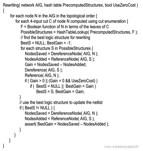
After trying all available subgraphs, the one that leads to the largest improvement at a node is used at the node. If there is no improvement but “zero-cost replacement” is enabled, a new subgraph that does not increase the number of nodes is used.
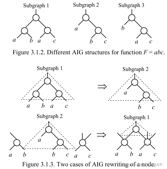
- Example
Example. Figure 3.1.2 shows three AIG subgraphs for the function F = abc. They are pre-computed and stored. Figure 3.1.3 shows two instances of AIG rewriting. The upper part of the figure shows the situation when Subgraph 1 is detected in the circuit and replaced by Subgraph 2. The lower part of the figure shows two nodes AND(a, b) and AND(a, c) already present in the network. In this case, Subgraph 2 can be replaced by Subgraph 1. In both cases, the network has one node less.
Resubstitution
- what is resubstitution ?
对于当前节点,重新使用网络中已经出现过的节点进行表示(真值值相同),如果在某些方面,例如节点数或者depth取得更好的效果,就会被接受。
Resubstitution expresses the function of a node using other nodes (called divisors) already present in the network. The transformation is accepted if the new implementation of the node is in some sense better than its current implementation using the immediate fanins.
- Some backgrounds
In the case of an AIG, the best outcome of resubstitution is when the whole MFFC of the node can be freed and the node’s function can be expressed using other nodes, currently outside of the node’s MFFC. This outcome corresponds to a 0-resubstitution when no new nodes are added to the AIG while the MFFC is removed. Similarly, if the MFFC is composed of more than one node, and there is no 0 resubstitution, the best outcome is given by a 1 resubstitution, which exists if the function of the node, whose MFFC is being considered, can be expressed using the available node and exactly one additional node.
- re-substitution example
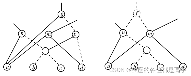
In the AIG shown in Figure 3.2.2 (left), node g has MFFC of size 2 composed of nodes g and p. One node can be saved if node g is replaced by the complement of node f, which does not belong to the original AIG but can be added on top of the already present nodes n and m, as shown in Figure 3.2.2 (right). Indeed, g = a(b + c + d), f = n + m = a(b + c) + ad = a(b + c + d). This resubstitution is an example of applying the algebraic distributive transform.
Redundancy removal
#TODO
2.2.5 Results
#TODO
2.3 Rewriting
paper: DAG-aware AIG rewriting: A fresh look at combinational logic synthesis, Alan, 2006.
#TODO
3. 储备知识
3.1 what is blif ?
伯克利实验室提出的一种表示逻辑电路的方法。
The goal of BLIF is to describe a logic-level hierarchical circuit in textual form.
- example
.names v3 v6 j u78 v13.15
1–0 1
-1-1 1
0-11 1
释义如下,
In a given row of the single-output-cover, “1” means the input is used in uncomplemented form, “0” means the input is complemented, and “–” means not used. Elements of a row are AND ed together, and then all rows are OR ed.
The translation of the above sample logic-gate into a sum-of-products notation would be as follows:
v13.15 = (v3 u78’) + (v6 u78) + (v3’ j u78)
To assign the constant “0” to some logic gate j, use the following construct:
.names j
To assign the constant “1”, use the following:
.names j
1
这里只给出了很基本的一种组合逻辑blif格式,如果想了解更多关于blif的内容,请参考文章:Berkeley Logic Interchange Format ( BLIF )
3.2 setup time和hold time
请参考本人另外一篇博客: setup time和hold time
3.3 弄懂时序逻辑
部分内容转自
一文详解时序逻辑
基本RS触发器(推荐)
组合电路是根据当前输入信号的组合来决定输出电平的电路,换言之,就是现在的输出不会被过去的输入所左右,也可以说成是,过去的输入状态对现在的输出状态没有影响的电路。
时序电路和组合电路不同,时序电路的输出不仅受现在输入状态的影响,还要受过去输入状态的影响。
那么,如何才能将过去的输入状态反映到现在的输出上呢?时序电路到底需要些什么呢?
人类总是根据过去的经验,决定现在的行动,这时我们需要的就是—记忆,同样时序电路也需要这样的功能,这种能够实现人类记忆功能的元器件就是触发器。
按结构和功能,触发器可以分为RS型、JK型、D型和T型,在这里,我们只讲解比较有代表性的类型,RS型和D型。
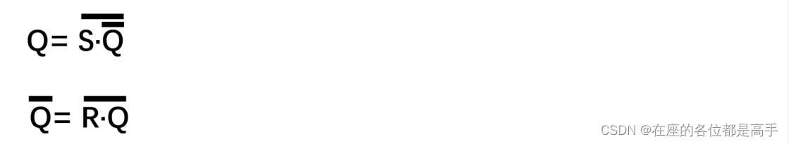
3.3.1 RS 触发器
- 电路图:

基本含义:
S是Set 的首字母,也就是设置端,R 是Reset 的首字母,也就是复位端。
触发器属于时序逻辑电路,与组合逻辑电路不同,组合逻辑电路的输出状态只取决于同时刻的输入信号状态。基本RS触发器把输出信号引回到输入信号,形成一个反馈。这样使得输出信号的状态不但取决于同时刻输入信号的状态,也与输出之前的状态有关。
输出信号的状态就是(Q^(N+1) 次态) 同时刻输入信号的状态就是(S、R) 输出之前的状态就是(Q^N 现态)
- 真值表
H/L代表高/低电平,初始态:Q=L、Q#=H、R=L、S=L,表中Q0和Q0#表示的是输入变化以前的输出,RS触发器是最简单的触发器,主要用于防止机械式开关的误操作。:
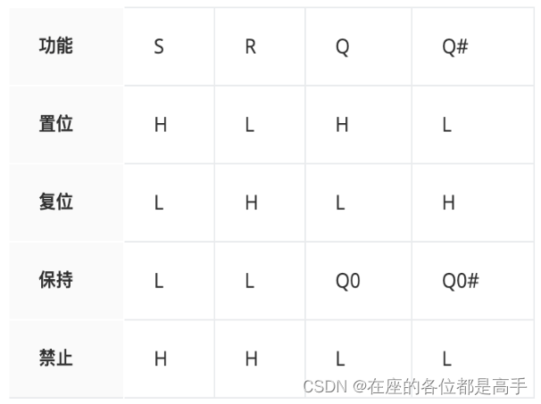
对照逻辑表达式和真值表更容易记忆:
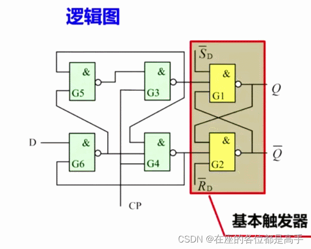
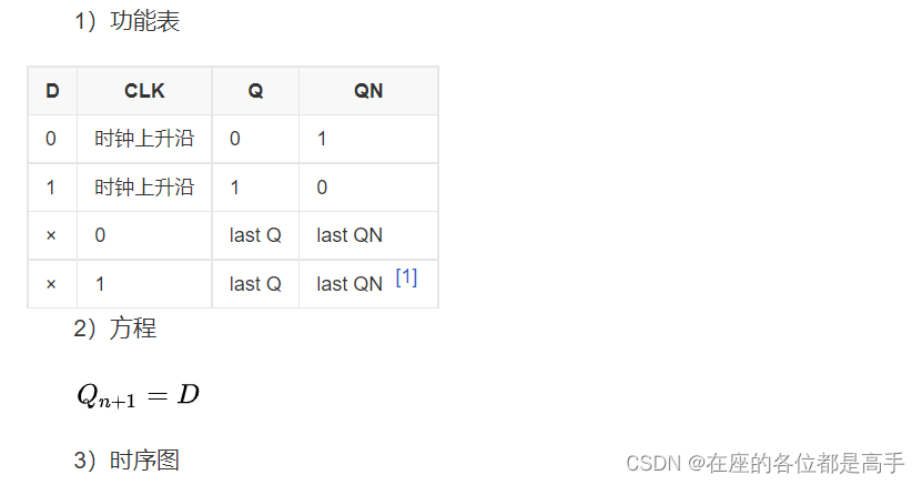
3.3.2 D触发器(A Flip Flop, DFF)
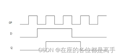
D触发器的工作原理:在一个脉冲信号(一般为晶振产生的时钟脉冲)上升沿或下降沿的作用下,将信号从输入端D送到输出端Q,如果时钟脉冲的边沿信号未出现,即使输入信号改变,输出信号仍然保持原值。
对应真值表和表达式可以更好理解,摘自百度百科。
3.3.3 寄存器
由于触发器内由记忆功能,因此可以利用触发器方便的构成寄存器。由于一个触发器能够存储一位二进制码,所以把n个触发器的时钟端口连接起来就能构成一个存储n位二进制码的寄存器。
按照功能的不同,可将寄存器分为基本寄存器和移位寄存器两大类。基本寄存器只能并行送入数据,也只能并行输出。移位寄存器中的数据可以在移位脉冲作用下依次逐位右移或左移,数据既可以并行输入、并行输出,也可以串行输入、串行输出,还可以并行输入、串行输出,或串行输入、并行输出,十分灵活,用途也很广。
More details u can refer to this presentation [寄存器讲解]
3.4 mux & decoder & selector
请参考本人这篇博客 ,
mux & decoder & selector详解
3.5 HVT/SVT/LVT
请参考本人这篇博客,
HVT/SVT/LVT详解
3.6 逻辑优化基础-strash
请参考本人这篇博客,
逻辑优化基础-strash
3.7 逻辑优化基础-rewrite
请参考本人这篇博客,
逻辑优化基础-rewrite
3.8 逻辑优化基础-cofactor
请参考本人这篇博客,
逻辑优化基础-cofactor
3.9 逻辑优化基础-shannon decomposition(详细版)
请参考本人这篇博客,
逻辑优化基础-shannon decomposition


 7802
7802


 被折叠的 条评论
为什么被折叠?
被折叠的 条评论
为什么被折叠?
 到【灌水乐园】发言


