【深度学习】利用Logistic回归函数识别猫

最新推荐文章于 2024-07-09 21:50:49 发布

射手座狗主

最新推荐文章于 2024-07-09 21:50:49 发布

阅读量772

点赞数 4

分类专栏：深度学习文章标签：逻辑回归深度学习

本文链接：https://blog.csdn.net/weixin_44410494/article/details/103378150

版权

深度学习专栏收录该内容

1 篇文章 0 订阅

订阅专栏

【深度学习】利用Logistic回归函数识别猫

这是博主学习完吴恩达视频后完成课后作业的一点感悟，想把数据保留下来故发了一篇博客，参考：【Kullbear】的GitHub文章

数据集请用百度网盘下载：点击下载提取码：e1om，其中lr_utils.py是读取datasets的函数，本人直接整合到一起了所以实际上也用不上了，完整代码在文章最下方。datasets的是数据集，请确保放在代码同目录下。

深度学习课后编程作业：具有神经网络思维的Logistic回归

logistic回归又称logistic回归分析，是一种广义的线性回归分析模型，可用于各种领域，包括机器学习，大多数医学领域和社会科学。例如，最初由Boyd等人开发的创伤和损伤严重程度评分（TRISS）被广泛用于预测受伤患者的死亡率，基于观察到的患者特征（年龄，性别，体重指数），使用逻辑回归分析预测发生特定疾病（例如糖尿病，冠心病）的风险，各种结果验血等。另一个例子可能是根据年龄，收入，性别，种族，居住状况，前次选举的投票等来预测尼泊尔选民是否将投票给尼泊尔国会或尼泊尔共产党或任何其他政党。所述的技术也可以在使用的工程，尤其是用于预测给定的过程中，系统或产品的故障的可能性。还用于市场营销应用程序，例如预测客户购买产品或中止订购的倾向等。在经济学中它可以用来预测一个人选择进入劳动力市场的可能性，而商业应用则可以用来预测房主拖欠抵押贷款的可能性。条件随机字段是逻辑回归到顺序数据的扩展，用于自然语言处理。

根据上面的例子可以看出，logistic函数主要通过一些自变量（年龄、性别等参数）线性组合得到一个事件的值（是否患病的结果），这里的自变量可以是二进制变量（两个类，由指示符变量编码）或连续变量（任何实数值），其中就包括图片的格式（三维数组），所以不难理解可以拿logistic函数来识别图片，并且识别图片还是比较简单的logistic函数应用。

利用logistic函数【识别猫】

并用自己的图片验证预测是否准确

import numpy as np
import matplotlib.pyplot as plt
import h5py
# import scipy
# from PIL import Image
# from scipy import ndimage
import imageio
import skimage

导入所需要的库，不多说，注释的因python版本或编译器而异，如果去掉可能出错，自己导包即可，本人用的python3.7，anaconda管理导入的包。

def load_dataset():
    train_dataset = h5py.File('datasets/train_catvnoncat.h5',"r")
    train_set_x_orig = np.array(train_dataset["train_set_x"][:])
    train_set_y_orig = np.array(train_dataset["train_set_y"][:])

    test_dataset = h5py.File('datasets/test_catvnoncat.h5',"r")
    test_set_x_orig = np.array(test_dataset["test_set_x"][:])
    test_set_y_orig = np.array(test_dataset["test_set_y"][:])

    classes = np.array(test_dataset["list_classes"][:])

    train_set_y_orig = train_set_y_orig.reshape((1, train_set_y_orig.shape[0]))
    test_set_y_orig = test_set_y_orig.reshape((1, test_set_y_orig.shape[0]))

    return train_set_x_orig, train_set_y_orig, test_set_x_orig, test_set_y_orig, classes

train_set_x_orig, train_set_y, test_set_x_orig, test_set_y, classes = load_dataset()

将读取文件的方式写成了方法，定义的参数也比较好理解，最后用参数接收方法里面返回的值。

train_set_x_orig/ test_set_x_orig ：保存的是训练集/测试集里面的图片数据。
train_set_y_orig ：保存的是训练集/测试集对图片的定义，0表示不是猫，1表示是猫。
classes保存的是以bytes类型保存的两个字符串数据[‘cat’,‘non-cat’]。

读取到文件后我们可以简单看一下数据集的内容。

index = 2
plt.imshow(train_set_x[index])
plt.show()
print("train_set_y = " + str(train_set_y))
print("y=" + str(train_set_y[:, index]) + ", it's a " + classes[np.squeeze(train_set_y[:, index])].decode("utf-8") + "'picture")

m_train = train_set_y.shape[1]  # 训练集里图片的数量。
m_test = test_set_y.shape[1]  # 测试集里图片的数量。
num_px = train_set_x_orig.shape[1]  # 训练、测试集里面的图片的宽度和高度（均为64x64）。

# 现在看一看我们加载的东西的具体情况
print ("训练集的数量: m_train = " + str(m_train))
print ("测试集的数量 : m_test = " + str(m_test))
print ("每张图片的宽/高 : num_px = " + str(num_px))
print ("每张图片的大小 : (" + str(num_px) + ", " + str(num_px) + ", 3)")
print ("训练集_图片的维数 : " + str(train_set_x_orig.shape))
print ("训练集_标签的维数 : " + str(train_set_y.shape))
print ("测试集_图片的维数: " + str(test_set_x_orig.shape))
print ("测试集_标签的维数: " + str(test_set_y.shape))

根据结果：
定义index，plt.imshow（train_set_x[index]）方法打印查看第index+1张图片。有的编译器如jupyter可以不用加plt.show()，视情况而定。
可以看到当我们用index=2时，我们查看的是第三张图片，第三个图片是一只猫，数组第三位是1，并且输出为cat，也可以自己查看其他图片。
在这里插入图片描述

打印出数据集的其他参数，数据集中训练集/测试集有图片209/50张，图片的参数为6464，3代表的是一个图片像素是由三原色组成的，每个原色是一个不同的数，故一张图片是6464*3的三维数组。

对于这种数据我们将它转换成一维数组来处理，np.reshape()方法reshape（m，n）的作用是将数组重组成m行n列，-1表示自动计算行列，最后得到的是一个n行1列的一维数组，因为在numpy中列的向量更容易计算，故转置成n列1行的一个数组。将本来是209个三维的一个数据转换成12288行109列的数据。

train_set_x_flatten = train_set_x_orig.reshape(train_set_x_orig.shape[0], -1).T
test_set_x_flatten = test_set_x_orig.reshape(test_set_x_orig.shape[0], -1).T

print("训练集降维最后的维度： " + str(train_set_x_flatten.shape))
print("训练集_标签的维数 : " + str(train_set_y.shape))
print("测试集降维之后的维度: " + str(test_set_x_flatten.shape))
print("测试集_标签的维数 : " + str(test_set_y.shape))

最后可以打印查看结果：
在这里插入图片描述
前面说到三原色，三原色以不同的比例相加，以产生多种多样的颜色，转换成一维数组后连续的3个数代表的是一个像素的色彩，计算机用8位2进制数表示颜色，所以数组中所有的值都在[0,255]之间，跟150分制现在要转换成百分制的时候除以150的道理一样，为了规范化就要除以255，所得的结果在[0，1]之间。

train_set_x = train_set_x_flatten/255
test_set_x = test_set_x_flatten/255

如图，将一个图片转换成12288个这样的元，计算每个元的权重和偏置值：
$z^{(i)} = w^T x^{(i)} + b \tag{1}$
$\hat{y}^{(i)} = a^{(i)} = sigmoid(z^{(i)})\tag{2}$
$\mathcal{L}(a^{(i)}, y^{(i)}) = - y^{(i)} \log(a^{(i)}) - (1-y^{(i)} ) \log(1-a^{(i)})\tag{3}$

公式(1)计算的是元的一个输入的值，总的输入的值是z⁽¹⁾+z⁽²⁾+····+z⁽ⁱ⁾+····z^(12288)，再通过元的激励函数(公式2)如ReLU或者sigmoid函数等，计算元的输出，根据输出的结果判定是否为猫（概率超过0.5的记为1判定有猫，相反则记0没猫）。
公式(3)是损失函数，损失函数衡量的是预测的y’与实际y之间的关系，通过损失函数来让w，b学习，得到最好的w和b使结果更优。
下图是sigmoid函数的图形。

定义sigmoid函数：

def sigmoid(z):
    s = 1/(1 + np.exp(-z))
    return s

初始化权重w，偏置b:
定义一个全0的numpy数组，dim作为虚参在后面传入的是图片的数组大小，zeros根据图片的数组初始一个与图片数组大小一致的全0数组w，偏置值b设为0。

def initialize_with_zeros(dim):
    w = np.zeros(shape=(dim, 1))
    b = 0
    assert(w.shape == (dim, 1))
    assert(isinstance(b, float) or isinstance(b, int))
    return (w, b)

w，b设置好之后就应该如图一样传播，传播的目的是计算总的损失函数，并且定义成本函数，成本函数是损失函数和比x的个数。

损失函数是对一个x的y’，成本函数是对所有的x的y’
$\frac{1}{m} \sum_{i=1}^m \mathcal{L}(a^{(i)}, y^{(i)})\tag{6}$
下面代码中正向传播的A实际上就是元对这张图片的预测值也就是输出值y’，与真正的y(y就是代表了有猫或者没猫的0或者1)形成的一个非线性关系，当输入的是有猫的图时y’就要尽可能的等于y=1，没猫时y’就要尽可能的等于y=0，公式(3)(4)就是万能的数学家想出来的这个关系的函数表示。这种表示可以得到一个处处可导的凹状曲线以确定一个对数据集最优的预测y’也就是成本函数。
当w，b不在最优时我们需要根据梯度来调整w和b，那么给出当前梯度(导数)dw和db，当后面不在最优时通过学习率*导数的方法改变w，b，也称为反向传播。

grads是定义一个集合，存放导数。

def propagate(w, b, X, Y):
    m = X.shape[1]

    # 正向传播
    A = sigmoid(np.dot(w.T, X) + b)
    # 计算成本
    cost = (-1 / m) * np.sum(Y * np.log(A) + (1 - Y)*(np.log(1 - A)))

    # 反向传播
    dw = (1 / m) * np.dot(X, (A - Y).T)
    db = (1 / m) * np.sum(A - Y)

    assert (dw.shape == w.shape)
    assert (db.dtype == float)
    cost = np.squeeze(cost)
    assert (cost.shape == ())

    grads = {
        "dw": dw,
        "db": db
    }
    return (grads, cost)

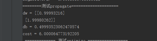
写好之后我们可以测试一下：

print("========测试propagate====================")
w, b, X, Y = np.array([[1], [2]]), 2, np.array([[1, 2], [3, 4]]), np.array([[1, 0]])
grads, cost = propagate(w, b, X, Y)
print("dw = " + str(grads["dw"]))
print("db = " + str(grads["db"]))
print("cost = " + str(cost))

得到结果：取的w，b，X，Y都比较简单并且算出来的数也刚好是整数，可以手动验证，本人取e=2.71828182得到的A= |1，1|，dw是[1,2]，db = 0.5，与结果一致，成本的计算也可以验证。
在这里插入图片描述
当把传播的步骤写好之后要让网络能够自己学习有更好的w，b，通过成本函数让w和b梯度下降到最优值，下面是优化的方法：
其中α是学习率，θ就是w，b。
$\theta = \theta - \alpha \text{ } d\theta$

代码为：
初始w，b都为0但dw，db的结果是不为0的，当定义了学习率之后w，b就会变化，引起dw，db的变化，循环直到为0时代表已经在凹曲线最底端，学习到了最好的w，b（不同的学习率对w，b有影响）。

ef optimize(w, b, X, Y, num_iterations, learning_rate, print_cost=False):
    costs = []

    for i in range(num_iterations):
        grads, cost = propagate(w, b, X, Y)

        dw = grads["dw"]
        db = grads["db"]

        w = w - learning_rate * dw
        b = b - learning_rate * db

        if i % 100 == 0:
            costs.append(cost)
        if (print_cost) and (i % 100 == 0):
             print("迭代的次数: %i,误差值:%f" % (i, cost))

    params = {
        "w": w,
        "b": b
    }
    grads = {
        "dw": dw,
        "db": db
    }
    return (params,grads,costs)

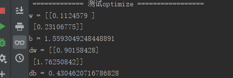
可以写测试代码验证，测试代码及结果为：

print(" {} ".format(str("============= 测试optimize =================")))
w, b, X, Y = np.array([[1], [2]]), 2, np.array([[1, 2], [3, 4]]), np.array([[1, 0]])
params, grads, costs = optimize(w, b, X, Y, num_iterations=100, learning_rate=0.009, print_cost=False)
print("w = " + str(params["w"]))
print("b = " + str(params["b"]))
print("dw = " + str(grads["dw"]))
print("db = " + str(grads["db"]))

在这里插入图片描述
优化函数完成之后开始对输出的值A进行预测，构造的Y_predoction(prediction拼写错了，小问题)是与A相同行列的数组，当A的值大于0.5时就置为1，小于则置为0，经典二分类方法。

def predict(w, b, X):
    m = X.shape[1]
    Y_predoction = np.zeros((1, m))
    w = w.reshape(X.shape[0], 1)

    A = sigmoid(np.dot(w.T, X) + b)
    for i in range(A.shape[1]):
        Y_predoction[0, i] = 1 if A[0, i] > 0.5 else 0

    assert(Y_predoction.shape == (1, m))
    return Y_predoction

所有方法已经构造好了，可以整合到一个模型方法中进行实际应用了，下面定义model方法。
写完之后我们已经可以用model方法对我们的数据集进行分辨了。

def model(X_train, Y_train, X_test, Y_test, num_iterations = 2000, learning_rate = 0.5, print_cost = False):
    w, b = initialize_with_zeros(X_train.shape[0])

    parameters, grads, costs = optimize(w, b, X_train, Y_train, num_iterations, learning_rate, print_cost)

    w, b = parameters["w"], parameters["b"]
    Y_prediction_test = predict(w, b, X_test)
    Y_prediction_train = predict(w, b, X_train)
    print("训练集准确性:", format(100 - np.mean(np.abs(Y_prediction_train - Y_train)) * 100), "%")
    print("测试集准确性:", format(100 - np.mean(np.abs(Y_prediction_test - Y_test)) * 100), "%")

    precise = 100 - np.mean(np.abs(Y_prediction_test - Y_test)) * 100


    d = {
        "costs": costs,
        "Y_prediction_test": Y_prediction_test,
        "Y_prediction_train": Y_prediction_train,
        "w": w,
        "b": b,
        "learning_rate": learning_rate,
        "num_iterations": num_iterations,
        "precise": precise
    }
    return d

print("=============测试model========================")
d = model(train_set_x, train_set_y, test_set_x, test_set_y, num_iterations=2000, learning_rate=0.005, print_cost=True)

结果为：
可以改变学习率或者迭代次数来查看测试的准确性，本人最高测试准确性达到75%，用一个简单的logistic函数并且没有神经网络的结构能到这么高也很神奇了。
在这里插入图片描述
对于上面的效果可以用plt画出来，显示如下：

costs = np.squeeze(d['costs'])
plt.plot(costs)
plt.ylabel('cost')
plt.xlabel('iterations(per hundreds)')
plt.title("Learning rate = " + str(d["learning_rate"]))
plt.show()

在这里插入图片描述

除此之外，我们能在一张图上画出不同的学习率对迭代次数的曲线，代码如下，选取的学习率可以自己多试验几次，本人只做了3个学习率的曲线，因为一条学习率的曲线就要迭代2000次，时间复杂度成比例增加，怕电脑扛不住所以就没多设。

learning_rates = [0.01, 0.001, 0.0001]
models = {}
for i in learning_rates:
    print("leaning rate is :" + str(i))
    models[str(i)] = model(train_set_x, train_set_y, test_set_x, test_set_y, num_iterations=1500, learning_rate= i , print_cost=False)
    print('\n' + "===========================")

for i in learning_rates:
    plt.plot(np.squeeze(models[str(i)]["costs"]), label = str(models[str(i)]["learning_rate"]))

plt.ylabel('cost')
plt.xlabel('iterations')
legend = plt.legend(loc='upper center', shadow=True)
frame = legend.get_frame()
frame.set_facecolor('0.90')
plt.show()

在这里插入图片描述

既然可以画出学习率对迭代次数的影响的影响，那么可否考虑学习率对准确性的影响呢，当很多的学习率对准确性的点连起来之后不就是一个曲线嘛，那就能看到最高的准确性时学习率是多少了。
作一个等差递增数组，尽可能多的画点。
画了几点看看效果，学习率上升再下降，可能是过拟合造成的，代码附上，大佬设备好一点的尽可以实现。

# precise随着learning_rate的变化曲线图可用此得到
learning_rates = np.arange(0.0001, 0.01, 0.002)
models = {}
for i in learning_rates:
    models[str(i)] = model(train_set_x, train_set_y, test_set_x, test_set_y, num_iterations=1500, learning_rate=i, print_cost=False)

for i in learning_rates:
    costs = models[str(i)]['precise']
    plt.plot(i, costs, 'ro')
plt.ylabel('precise')
plt.xlabel('learning_rate')
plt.show()

在这里插入图片描述
最后我们用可以自己找的图片来验证是否是猫，代码如下：
说两点：
1.深度学习视频上用的是ndimage.imread方法，但更新之后换到新的imageio库中，用imageio.imread方法。
2.深度学习视频中用的是scipy.misc.imresize方法，更新之后换到新的skimage库中，用skimage.transform.resize方法。

my_image = "myimage3.jpg"

image = np.array(imageio.imread(my_image))
my_image = skimage.transform.resize(image, (num_px, num_px)).reshape((1, num_px * num_px*3)).T
my_predict_image = predict(d["w"], d["b"],my_image)
plt.imshow(image)
plt.show()
print("y = " + str(np.squeeze(my_predict_image)) + ", your algorithm predicts a \"" + classes[int(np.squeeze(my_predict_image)),].decode("utf-8") + "\" picture.")

问题不大，验证如下：
在这里插入图片描述

完整代码：

import numpy as np
import matplotlib.pyplot as plt
import h5py
import scipy
# from lr_utils import load_dataset
from PIL import Image
from scipy import ndimage
import imageio
import skimage

def load_dataset():
    train_dataset = h5py.File('datasets/train_catvnoncat.h5',"r")
    train_set_x_orig = np.array(train_dataset["train_set_x"][:])
    train_set_y_orig = np.array(train_dataset["train_set_y"][:])

    test_dataset = h5py.File('datasets/test_catvnoncat.h5',"r")
    test_set_x_orig = np.array(test_dataset["test_set_x"][:])
    test_set_y_orig = np.array(test_dataset["test_set_y"][:])

    classes = np.array(test_dataset["list_classes"][:])

    train_set_y_orig = train_set_y_orig.reshape((1, train_set_y_orig.shape[0]))
    test_set_y_orig = test_set_y_orig.reshape((1, test_set_y_orig.shape[0]))

    return train_set_x_orig, train_set_y_orig, test_set_x_orig, test_set_y_orig, classes


train_set_x_orig, train_set_y, test_set_x_orig, test_set_y, classes = load_dataset()


index = 2
plt.imshow(train_set_x_orig[index])
plt.show()
print("train_set_y = " + str(train_set_y))
print("y=" + str(train_set_y[:, index]) + ", it's a " + classes[np.squeeze(train_set_y[:, index])].decode("utf-8") + "'picture")

m_train = train_set_y.shape[1]  # 训练集里图片的数量。
m_test = test_set_y.shape[1]  # 测试集里图片的数量。
num_px = train_set_x_orig.shape[1]  # 训练、测试集里面的图片的宽度和高度（均为64x64）。

# 现在看一看我们加载的东西的具体情况
print ("训练集的数量: m_train = " + str(m_train))
print ("测试集的数量 : m_test = " + str(m_test))
print ("每张图片的宽/高 : num_px = " + str(num_px))
print ("每张图片的大小 : (" + str(num_px) + ", " + str(num_px) + ", 3)")
print ("训练集_图片的维数 : " + str(train_set_x_orig.shape))
print ("训练集_标签的维数 : " + str(train_set_y.shape))
print ("测试集_图片的维数: " + str(test_set_x_orig.shape))
print ("测试集_标签的维数: " + str(test_set_y.shape))

train_set_x_flatten = train_set_x_orig.reshape(train_set_x_orig.shape[0], -1).T
test_set_x_flatten = test_set_x_orig.reshape(test_set_x_orig.shape[0], -1).T

print("训练集降维最后的维度： " + str(train_set_x_flatten.shape))
print("训练集_标签的维数 : " + str(train_set_y.shape))
print("测试集降维之后的维度: " + str(test_set_x_flatten.shape))
print("测试集_标签的维数 : " + str(test_set_y.shape))


train_set_x = train_set_x_flatten/255
test_set_x = test_set_x_flatten/255


def sigmoid(z):
    s = 1/(1 + np.exp(-z))
    return s

# print("========测试sigmoid===============================")
# print("sigmoid(0) = " + str(sigmoid(0)))
# print("sigmoid(9.2) = " + str(sigmoid(9.2)))

def initialize_with_zeros(dim):
    w = np.zeros(shape=(dim, 1))
    b = 0
    assert(w.shape == (dim, 1))
    assert(isinstance(b, float) or isinstance(b, int))
    return (w, b)

def propagate(w, b, X, Y):
    m = X.shape[1]

    # 正向传播
    A = sigmoid(np.dot(w.T, X) + b)
    # 计算成本
    cost = (-1 / m) * np.sum(Y * np.log(A) + (1 - Y)*(np.log(1 - A)))

    # 反向传播
    dw = (1 / m) * np.dot(X, (A - Y).T)
    db = (1 / m) * np.sum(A - Y)

    assert (dw.shape == w.shape)
    assert (db.dtype == float)
    cost = np.squeeze(cost)
    assert (cost.shape == ())

    grads = {
        "dw": dw,
        "db": db
    }
    return (grads, cost)

print("========测试propagate====================")
w, b, X, Y = np.array([[1], [2]]), 2, np.array([[1, 2], [3, 4]]), np.array([[1, 0]])
grads, cost = propagate(w, b, X, Y)
print("dw = " + str(grads["dw"]))
print("db = " + str(grads["db"]))
print("cost = " + str(cost))


def optimize(w, b, X, Y, num_iterations, learning_rate, print_cost=False):
    costs = []

    for i in range(num_iterations):
        grads, cost = propagate(w, b, X, Y)

        dw = grads["dw"]
        db = grads["db"]

        w = w - learning_rate * dw
        b = b - learning_rate * db

        if i % 100 == 0:
            costs.append(cost)
        if (print_cost) and (i % 100 == 0):
             print("迭代的次数: %i,误差值:%f" % (i, cost))

    params = {
        "w": w,
        "b": b
    }
    grads = {
        "dw": dw,
        "db": db
    }
    return (params,grads,costs)

print(" {} ".format(str("============= 测试optimize =================")))
w, b, X, Y = np.array([[1], [2]]), 2, np.array([[1, 2], [3, 4]]), np.array([[1, 0]])
params, grads, costs = optimize(w, b, X, Y, num_iterations=100, learning_rate=0.009, print_cost=False)
print("w = " + str(params["w"]))
print("b = " + str(params["b"]))
print("dw = " + str(grads["dw"]))
print("db = " + str(grads["db"]))

def predict(w, b, X):
    m = X.shape[1]
    Y_predoction = np.zeros((1, m))
    w = w.reshape(X.shape[0], 1)

    A = sigmoid(np.dot(w.T, X) + b)
    for i in range(A.shape[1]):
        Y_predoction[0, i] = 1 if A[0, i] > 0.5 else 0

    assert(Y_predoction.shape == (1, m))
    return Y_predoction

print("=============测试predict=======================")
w, b, X, Y = np.array([[1], [2]]), 2, np.array([[1, 2], [3, 4]]), np.array([[1, 0]])
print("predictions = " + str(predict(w, b, X)))



def model(X_train, Y_train, X_test, Y_test, num_iterations = 2000, learning_rate = 0.5, print_cost = False):
    w, b = initialize_with_zeros(X_train.shape[0])

    parameters, grads, costs = optimize(w, b, X_train, Y_train, num_iterations, learning_rate, print_cost)

    w, b = parameters["w"], parameters["b"]
    Y_prediction_test = predict(w, b, X_test)
    Y_prediction_train = predict(w, b, X_train)
    print("训练集准确性:", format(100 - np.mean(np.abs(Y_prediction_train - Y_train)) * 100), "%")
    print("测试集准确性:", format(100 - np.mean(np.abs(Y_prediction_test - Y_test)) * 100), "%")

    precise = 100 - np.mean(np.abs(Y_prediction_test - Y_test)) * 100


    d = {
        "costs": costs,
        "Y_prediction_test": Y_prediction_test,
        "Y_prediction_train": Y_prediction_train,
        "w": w,
        "b": b,
        "learning_rate": learning_rate,
        "num_iterations": num_iterations,
        "precise": precise
    }
    return d
print("=============测试model========================")
d = model(train_set_x, train_set_y, test_set_x, test_set_y, num_iterations=2000, learning_rate=0.005, print_cost=True)

costs = np.squeeze(d['costs'])
plt.plot(costs)
plt.ylabel('cost')
plt.xlabel('iterations(per hundreds)')
plt.title("Learning rate = " + str(d["learning_rate"]))
plt.show()


learning_rates = [0.01, 0.001, 0.0001]
models = {}
for i in learning_rates:
    print("leaning rate is :" + str(i))
    models[str(i)] = model(train_set_x, train_set_y, test_set_x, test_set_y, num_iterations=1500, learning_rate= i , print_cost=False)
    print('\n' + "===========================")

for i in learning_rates:
    plt.plot(np.squeeze(models[str(i)]["costs"]), label = str(models[str(i)]["learning_rate"]))

plt.ylabel('cost')
plt.xlabel('iterations')
legend = plt.legend(loc='upper center', shadow=True)
frame = legend.get_frame()
frame.set_facecolor('0.90')
plt.show()



# precise随着learning_rate的变化曲线图可用此得到
learning_rates = np.arange(0.0001, 0.01, 0.002)
models = {}
for i in learning_rates:
    models[str(i)] = model(train_set_x, train_set_y, test_set_x, test_set_y, num_iterations=1500, learning_rate=i, print_cost=False)

for i in learning_rates:
    costs = models[str(i)]['precise']
    plt.plot(i, costs, 'ro')
plt.ylabel('precise')
plt.xlabel('learning_rate')
plt.show()

my_image = "myimage3.jpg"

image = np.array(imageio.imread(my_image))
my_image = skimage.transform.resize(image, (num_px, num_px)).reshape((1, num_px * num_px*3)).T
my_predict_image = predict(d["w"], d["b"],my_image)
plt.imshow(image)
plt.show()
print("y = " + str(np.squeeze(my_predict_image)) + ", your algorithm predicts a \"" + classes[int(np.squeeze(my_predict_image)),].decode("utf-8") + "\" picture.")