InceptionTime模型结构解读

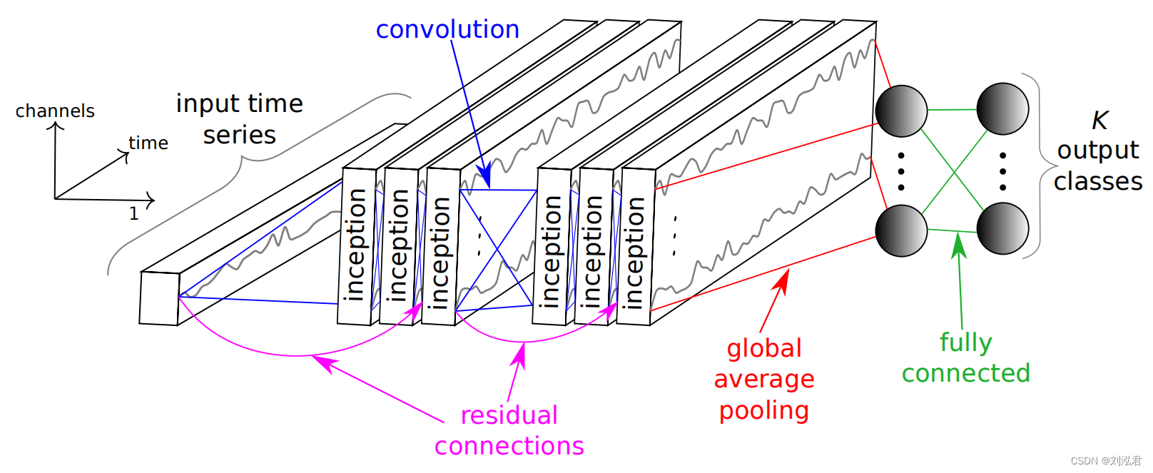
看一下模型init：

class Classifier_INCEPTION:

    def __init__(self, output_directory, input_shape, nb_classes, verbose=False, build=True, batch_size=64,
                 nb_filters=32, use_residual=True, use_bottleneck=True, depth=6, kernel_size=41, nb_epochs=1500):

        self.output_directory = output_directory

        self.nb_filters = nb_filters
        self.use_residual = use_residual
        self.use_bottleneck = use_bottleneck
        self.depth = depth
        self.kernel_size = kernel_size - 1
        self.callbacks = None
        self.batch_size = batch_size
        self.bottleneck_size = 32
        self.nb_epochs = nb_epochs

        if build == True:
            self.model = self.build_model(input_shape, nb_classes)
            if (verbose == True):
                self.model.summary()
            self.verbose = verbose
            self.model.save_weights(self.output_directory + 'model_init.hdf5')

可以发现，直接调用了self.build_model函数：

    def build_model(self, input_shape, nb_classes):
        # input_shape表示（输入时序数据的长度，输入数据的通道数），univariate的channel为1
        input_layer = keras.layers.Input(input_shape)

        x = input_layer
        input_res = input_layer

        # depth默认设置为6
        for d in range(self.depth):

            x = self._inception_module(x)

            # 当depth=2和depth=5时，分别进行残差传递
            if self.use_residual and d % 3 == 2:
                x = self._shortcut_layer(input_res, x)
                input_res = x

        gap_layer = keras.layers.GlobalAveragePooling1D()(x)

        # 表达式keras.layers.Dense(nb_classes, activation='softmax')(gap_layer)表示将gap_layer张量传递给Dense()层作为输入，并应用softmax激活函数生成输出张量。
        output_layer = keras.layers.Dense(nb_classes, activation='softmax')(gap_layer)

        model = keras.models.Model(inputs=input_layer, outputs=output_layer)

        model.compile(loss='categorical_crossentropy', optimizer=tf.keras.optimizers.Adam(),
                      metrics=['accuracy'])

        reduce_lr = keras.callbacks.ReduceLROnPlateau(monitor='loss', factor=0.5, patience=50,
                                                      min_lr=0.0001)

        file_path = self.output_directory + 'best_model.hdf5'

        model_checkpoint = keras.callbacks.ModelCheckpoint(filepath=file_path, monitor='loss',
                                                           save_best_only=True)

        self.callbacks = [reduce_lr, model_checkpoint]

        return model

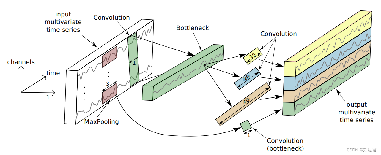
其中，_inception_module代码如下：

    def _inception_module(self, input_tensor, stride=1, activation='linear'):
        print('input',input_tensor.shape)
        if self.use_bottleneck and int(input_tensor.shape[-1]) > 1:
            input_inception = keras.layers.Conv1D(filters=self.bottleneck_size, kernel_size=1,
                                                  padding='same', activation=activation, use_bias=False)(input_tensor)
        else:
            input_inception = input_tensor
        print('inception',input_inception.shape)
        # kernel_size_s = [3, 5, 8, 11, 17]
        kernel_size_s = [self.kernel_size // (2 ** i) for i in range(3)]

        conv_list = []

        for i in range(len(kernel_size_s)):
            conv_list.append(keras.layers.Conv1D(filters=self.nb_filters, kernel_size=kernel_size_s[i],
                                                 strides=stride, padding='same', activation=activation, use_bias=False)(
                input_inception))

        max_pool_1 = keras.layers.MaxPool1D(pool_size=3, strides=stride, padding='same')(input_tensor)

        conv_6 = keras.layers.Conv1D(filters=self.nb_filters, kernel_size=1,
                                     padding='same', activation=activation, use_bias=False)(max_pool_1)

        conv_list.append(conv_6)

        x = keras.layers.Concatenate(axis=2)(conv_list)
        x = keras.layers.BatchNormalization()(x)
        x = keras.layers.Activation(activation='relu')(x)
        return x

这里放上原文：

As for the Inception module, Fig. 2 illustrates the inside details of this operation. Let us consider
the input to be an MTS with M dimensions. The first major component of the Inception module
is called the “bottleneck” layer. This layer performs an operation of sliding m filters of length 1
with a stride equal to 1. This will transform the time series from an MTS with M dimensions
to an MTS with m M dimensions, thus reducing significantly the dimensionality of the time
series as well as the model’s complexity and mitigating overfitting problems for small datasets.
Note that for visualization purposes, Fig. 2 illustrates a bottleneck layer with m = 1.

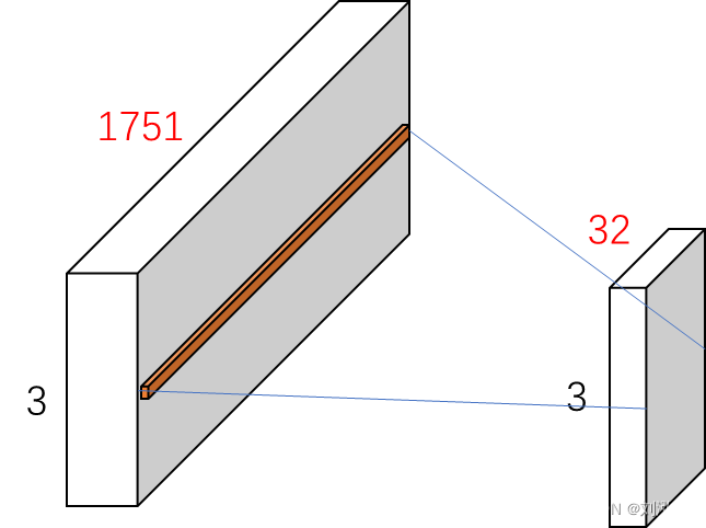
对于维度变化的理解：

假设此时我们有一个时序数据，3通道，长度1751

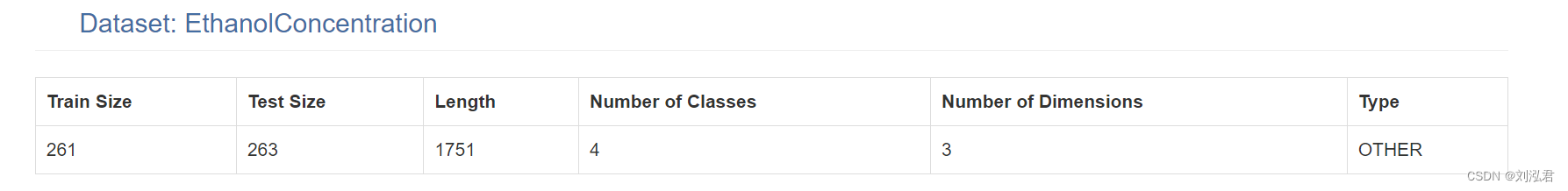
实验：在bottleneck中，设置filter_size=32，也就是滤波器数量32；经过bottleneck后，就变成了(3, 32)。

也就是说：在输入张量(input_tensor)的形状中，第一个维度(None)表示输入数据的数量未知，第二个维度(3)表示每个输入数据的通道数，而第三个维度(1751)表示每个通道的时间步数。因此，使用bottleneck设计的Conv1D层将时间步的特征数从1751降低到32，并保留通道数为3。输出张量(input_inception)的形状为(None, 3, 32)，其中32表示每个时间步的特征数被降低到了32，3表示每个输入数据的通道数被保留下来，而None表示输入数据的数量未知。
（所以图画的让人产生歧义）

对一维卷积的理解：

Conv1D层是对输入张量的第二个和第三个维度进行卷积操作的一种方式。在时序数据中，通常使用Conv1D层来处理时间序列的每个时间步，其中每个时间步的特征被视为一维数据。在Conv1D层中，滤波器沿着时间步轴滑动，并计算输入时间步的特征与滤波器之间的卷积运算，从而生成输出特征。

在代码中，Conv1D层的输入张量形状为(batch_size, timesteps, features)，其中batch_size是输入数据的数量，timesteps是时间步的数量，而features是每个时间步的特征数。Conv1D层的滤波器数量和大小由filters和kernel_size参数决定，padding和stride参数控制输出特征的大小和形状，activation和use_bias参数控制激活函数和是否使用偏置项。
（总觉得一维卷积的定义与实际当中的使用不太搭配，它相当于默认对第三维所有的值进行操作，kernel_size控制计算几个第二维（通道），参数filters控制第三维还剩下多少）

之后，就是拼起来，因此从32个特征变成了64个。
（代码里也没有体现论文中使用长度为40的卷积核）
根据我的理解，应该是这样子画图：

对于残差网络：

        input_res = input_layer

        # depth默认设置为6
        for d in range(self.depth):
            print(d)
            x = self._inception_module(x)

            # 当depth=2和depth=5时，分别进行残差传递
            if self.use_residual and d % 3 == 2:
                x = self._shortcut_layer(input_res, x)
                input_res = x
    def _shortcut_layer(self, input_tensor, out_tensor):
        shortcut_y = keras.layers.Conv1D(filters=int(out_tensor.shape[-1]), kernel_size=1,
                                         padding='same', use_bias=False)(input_tensor)
        shortcut_y = keras.layers.normalization.BatchNormalization()(shortcut_y)

        x = keras.layers.Add()([shortcut_y, out_tensor])
        x = keras.layers.Activation('relu')(x)
        return x

其中，x是inception学习的，也就是残差，input_res是作为初始值直接向后传递；但可以发现，input_res输入_shortcut_layer也要进行一个Conv1D也要进行学习。当然，他的目的可能是让特征长度一致。

附录：关于输入放在第二个括号中传入层

将输入张量作为第二个括号中的参数传递给Dense()函数，那么这是keras早期版本的语法。在早期版本中，可以通过将输入张量作为第二个参数传递来调用Dense()函数，例如：

output_layer = keras.layers.Dense(units=nb_classes, activation='softmax')(input_layer)

在这种情况下，input_layer是输入张量，它作为第二个参数传递给Dense()函数。这种方式仍然有效，但已被更新为更常见的函数式API，其中层被视为函数，并且可以像函数一样调用，将输入张量作为参数传递。

在更新的函数式API中，可以将输入张量作为第一个参数传递给Dense()函数，并将其结果传递给下一个层。例如：

dense_layer = keras.layers.Dense(units=64, activation='relu')
output_layer = dense_layer(input_layer)

在这种情况下，input_layer是输入张量，它作为第一个参数传递给Dense()函数，并将其结果存储在dense_layer变量中。可以继续将dense_layer作为输入传递给其他层或函数。