kaggle住房预测项目——第4部分(其他数据预处理方法)

kaggle住房预测项目——第4部分(其他数据预处理方法)

import numpy as np
import pandas as pd
%matplotlib inline
import matplotlib.pyplot as plt
import seaborn as sns
color = sns.color_palette()
sns.set_style('darkgrid')
from scipy import stats
from scipy.stats import norm, skew 

train = pd.read_csv('../data/train.csv')
test = pd.read_csv('../data/test.csv')

train.head(5)

	Id	MSSubClass	MSZoning	LotFrontage	LotArea	Street	Alley	LotShape	LandContour	Utilities	...	PoolArea	PoolQC	Fence	MiscFeature	MiscVal	MoSold	YrSold	SaleType	SaleCondition	SalePrice
0	1	60	RL	65.0	8450	Pave	NaN	Reg	Lvl	AllPub	...	0	NaN	NaN	NaN	0	2	2008	WD	Normal	208500
1	2	20	RL	80.0	9600	Pave	NaN	Reg	Lvl	AllPub	...	0	NaN	NaN	NaN	0	5	2007	WD	Normal	181500
2	3	60	RL	68.0	11250	Pave	NaN	IR1	Lvl	AllPub	...	0	NaN	NaN	NaN	0	9	2008	WD	Normal	223500
3	4	70	RL	60.0	9550	Pave	NaN	IR1	Lvl	AllPub	...	0	NaN	NaN	NaN	0	2	2006	WD	Abnorml	140000
4	5	60	RL	84.0	14260	Pave	NaN	IR1	Lvl	AllPub	...	0	NaN	NaN	NaN	0	12	2008	WD	Normal	250000

5 rows × 81 columns

test.head(5)

	Id	MSSubClass	MSZoning	LotFrontage	LotArea	Street	Alley	LotShape	LandContour	Utilities	...	ScreenPorch	PoolArea	PoolQC	Fence	MiscFeature	MiscVal	MoSold	YrSold	SaleType	SaleCondition
0	1461	20	RH	80.0	11622	Pave	NaN	Reg	Lvl	AllPub	...	120	0	NaN	MnPrv	NaN	0	6	2010	WD	Normal
1	1462	20	RL	81.0	14267	Pave	NaN	IR1	Lvl	AllPub	...	0	0	NaN	NaN	Gar2	12500	6	2010	WD	Normal
2	1463	60	RL	74.0	13830	Pave	NaN	IR1	Lvl	AllPub	...	0	0	NaN	MnPrv	NaN	0	3	2010	WD	Normal
3	1464	60	RL	78.0	9978	Pave	NaN	IR1	Lvl	AllPub	...	0	0	NaN	NaN	NaN	0	6	2010	WD	Normal
4	1465	120	RL	43.0	5005	Pave	NaN	IR1	HLS	AllPub	...	144	0	NaN	NaN	NaN	0	1	2010	WD	Normal

5 rows × 80 columns

print("The train data size before dropping Id feature is : {} ".format(train.shape))
print("The test data size before dropping Id feature is : {} ".format(test.shape))

#Save the 'Id' column
train_ID = train['Id']
test_ID = test['Id']

#Now drop the  'Id' colum since it's unnecessary for  the prediction process.
train.drop("Id", axis = 1, inplace = True)
test.drop("Id", axis = 1, inplace = True)

print("\nThe train data size after dropping Id feature is : {} ".format(train.shape)) 
print("The test data size after dropping Id feature is : {} ".format(test.shape))

The train data size before dropping Id feature is : (1460, 81) 
The test data size before dropping Id feature is : (1459, 80) 

The train data size after dropping Id feature is : (1460, 80) 
The test data size after dropping Id feature is : (1459, 79) 

数据预处理

异常值

fig, ax = plt.subplots()
ax.scatter(x = train['GrLivArea'], y = train['SalePrice'])
plt.ylabel('SalePrice', fontsize=13)
plt.xlabel('GrLivArea', fontsize=13)
plt.show()

#Deleting outliers
train = train.drop(train[(train['GrLivArea']>4000) & (train['SalePrice']<300000)].index)

#Check the graphic again
fig, ax = plt.subplots()
ax.scatter(train['GrLivArea'], train['SalePrice'])
plt.ylabel('SalePrice', fontsize=13)
plt.xlabel('GrLivArea', fontsize=13)
plt.show()

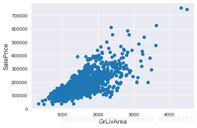
注意:注意移除异常值总是安全的。我们决定删除这两个，因为它们非常大，非常糟糕(非常大的区域，非常低的价格)。在训练数据中可能还有其他异常值。然而，如果在测试数据中也存在异常值，移除所有异常值可能会严重影响我们的模型。这就是为什么，我们不会把它们全部移除，而是设法让我们的一些模型在它们的基础上变得健壮。

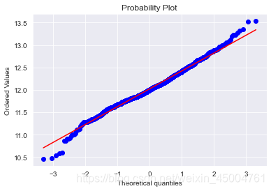
目标变量

SalePrice is the variable we need to predict. So let’s do some analysis on this variable first.

sns.distplot(train['SalePrice'] , fit=norm);

# Get the fitted parameters used by the function
(mu, sigma) = norm.fit(train['SalePrice'])
print( '\n mu = {:.2f} and sigma = {:.2f}\n'.format(mu, sigma))

#Now plot the distribution
plt.legend(['Normal dist. ($\mu=$ {:.2f} and $\sigma=$ {:.2f} )'.format(mu, sigma)],
            loc='best')
plt.ylabel('Frequency')
plt.title('SalePrice distribution')

#Get also the QQ-plot
fig = plt.figure()
res = stats.probplot(train['SalePrice'], plot=plt)
plt.show()

 mu = 180932.92 and sigma = 79467.79

​

目标变量是右偏的。由于(线性)模型喜欢正态分布的数据，我们需要对这个变量进行变换，使其更符合正态分布。

目标变量的对数变换

#We use the numpy fuction log1p which  applies log(1+x) to all elements of the column
train["SalePrice"] = np.log1p(train["SalePrice"]) # log1p = log（x+1）

#Check the new distribution 
sns.distplot(train['SalePrice'] , fit=norm);

# Get the fitted parameters used by the function
(mu, sigma) = norm.fit(train['SalePrice'])
print( '\n mu = {:.2f} and sigma = {:.2f}\n'.format(mu, sigma))

#Now plot the distribution
plt.legend(['Normal dist. ($\mu=$ {:.2f} and $\sigma=$ {:.2f} )'.format(mu, sigma)],
            loc='best')
plt.ylabel('Frequency')
plt.title('SalePrice distribution')

#Get also the QQ-plot
fig = plt.figure()
res = stats.probplot(train['SalePrice'], plot=plt)
plt.show()

 mu = 12.02 and sigma = 0.40

​

歪斜似乎得到了纠正，数据似乎更趋于正态分布。

特征工程

ntrain = train.shape[0]
ntest = test.shape[0]
y_train = train.SalePrice.values
all_data = pd.concat((train, test)).reset_index(drop=True)
all_data.drop(['SalePrice'], axis=1, inplace=True)
print("all_data size is : {}".format(all_data.shape))

all_data size is : (2917, 79)

缺失值处理

all_data_na = (all_data.isnull().sum() / len(all_data)) * 100
all_data_na = all_data_na.drop(all_data_na[all_data_na == 0].index).sort_values(ascending=False)[:30]
missing_data = pd.DataFrame({
   'Missing Ratio' :all_data_na})
missing_data.head(20)

	Missing Ratio
PoolQC	99.691464
MiscFeature	96.400411
Alley	93.212204
Fence	80.425094
FireplaceQu	48.680151
LotFrontage	16.660953
GarageFinish	5.450806
GarageYrBlt	5.450806
GarageQual	5.450806
GarageCond	5.450806
GarageType	5.382242
BsmtExposure	2.811107
BsmtCond	2.811107
BsmtQual	2.776826
BsmtFinType2	2.742544
BsmtFinType1	2.708262
MasVnrType	0.822763
MasVnrArea	0.788481
MSZoning	0.137127
BsmtFullBath	0.068564

f, ax = plt.subplots(figsize=(15, 12))
plt.xticks(rotation='90')
sns.barplot(x=all_data_na.index, y=all_data_na)
plt.xlabel('Features', fontsize=15)
plt.ylabel('Percent of missing values', fontsize=15)
plt.title('Percent missing data by feature', fontsize=15)

Text(0.5, 1.0, 'Percent missing data by feature')

数据相关性

#Correlation map to see how features are correlated with SalePrice
corrmat = train.corr()
plt.subplots(figsize=(12,9))
sns.heatmap(corrmat, vmax=0.9, square=True)

<matplotlib.axes._subplots.AxesSubplot at 0x2096d6a2b88>

• PoolQC: 数据描述中NA表示“无池”。考虑到巨大的缺失价值比率(+99%)和大多数房屋根本没有池子，这是有道理的。

all_data["PoolQC"] = all_data["PoolQC"].fillna("None")

• MiscFeature : data description says NA means “no misc feature”

all_data["MiscFeature"] = all_data["MiscFeature"].fillna("None")

• Alley : data description says NA means “no alley access”

all_data["Alley"] = all_data["Alley"].fillna("None")

• Fence : data description says NA means “no fence”

all_data["Fence"] = all_data["Fence"].fillna("None")

• FireplaceQu : data description says NA means “no fireplace”

all_data["FireplaceQu"] = all_data["FireplaceQu"].fillna("None")

• LotFrontage : 由于每条街道与房屋相连的区域很可能与邻近地区的其他房屋有相似的区域，我们可以通过该社区的中位数临街面积来填充缺失的值Since the area of each street connected to the house property most likely have a similar area to other houses in its neighborhood , we can fill in missing values by the median LotFrontage of the neighborhood.

#Group by neighborhood and fill in missing value by the median LotFrontage of all the neighborhood
all_data["LotFrontage"] = all_data.groupby("Neighborhood")["LotFrontage"].transform(
    lambda x: x.fillna(x.median()))

• GarageType, GarageFinish, GarageQual and GarageCond : Replacing missing data with None

for col in ('GarageType', 'GarageFinish', 'GarageQual', 'GarageCond'):
    all_data[col